Stat 414 – Review Problem Solutions (F24)

Let me know if you spot errors or want an answer elaborated on!

1) Plots

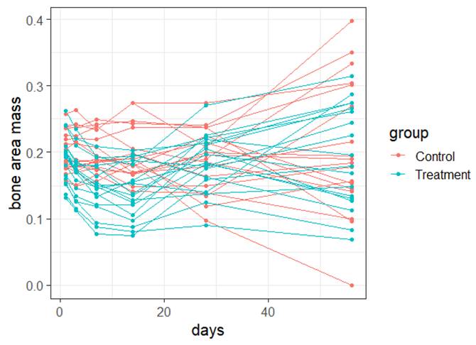
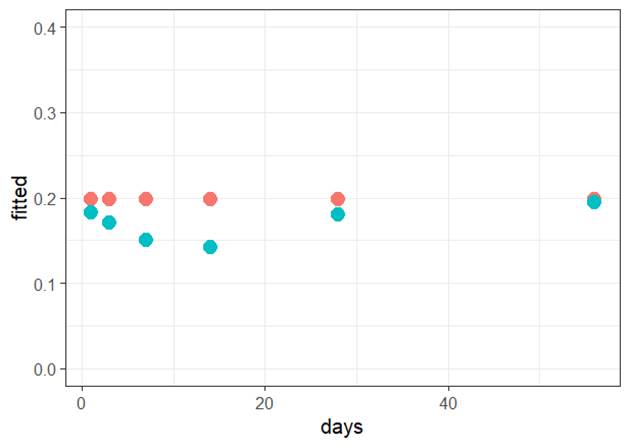
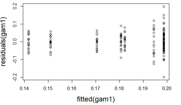
(a) Form of the model: Because the residuals vs. fits graph does not show any leftover pattern, the form of the model I used appears to be adequate.

Independence: We have repeated observations on the same mouse so independence is violated.

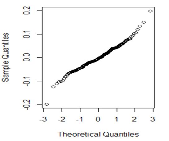
Normality: The normal probability plot looks reasonably linear, so the normality of the errors condition is met.

Equal variance: The residuals vs. fits graph shows increasing variability in the residuals with increasing fitted values, indicating a violation of equality of the error variances at each x (though not super severe)

(b) Which of the following would you consider doing next to improve the validity of the model? Briefly justify your choice(s).

· Transformation to improve linearity No, model form was fine.

· Quadratic model to improve linearity No, model form was fine

· Transformation of response to improve normality No, normality was fine

· Transformation of explanatory to improve normality No, normality was fine

· Include days as a variance covariate Yes, the variability in the residuals appears to increase with the number of days

· Include group as a variance covariate No, the variability in the two treatment groups appears reasonably equal

· Multilevel model using mouse as a grouping variable (Level 2 units) Yes, this will allow us to model the repeat observations over time as well as on each mouse (two knees)

2) Here is another model for the FEV data

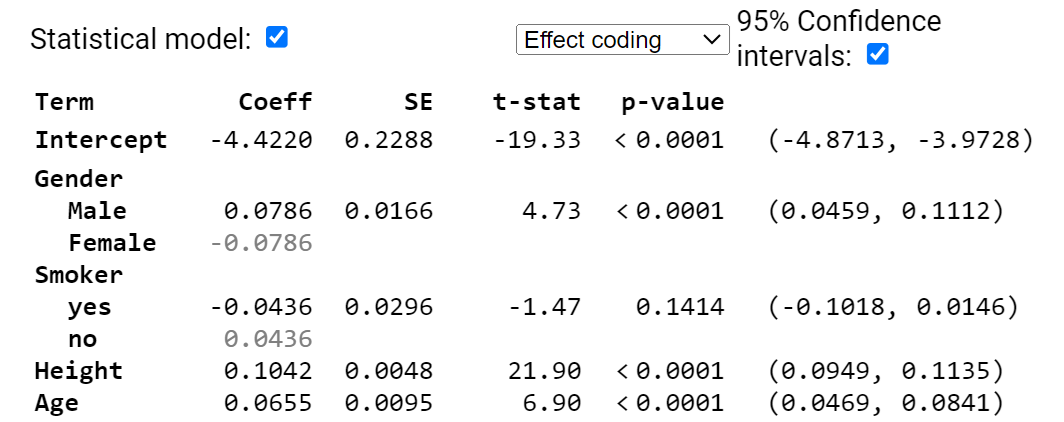
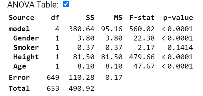
(a) Provide a rough estimate of a 95% confidence interval for a 17-year-old male smoker who is 64 inches tall.

First, we predict a 17-year-old male smoker, 64 inches

liters

Then a rough standard error around this prediction (for an individual) is 2 * residual standard error. Where do I find the residual standard error in the above output? = .412

I am 95% confident that an individual with these characteristics will have an FEV between 2.58 and 4.22.

From R

(b) Interpret the (0.0459, 0.1112) interval in context.

We are 95% confident that, after adjusting for height, smoking status, and age, the average FEV of males is 0.0459 to 0.112 liters higher than average (or about .09 to .22 liters higher than the females average of the same age, height, and smoking status).

Note, with this “complete output” I can see that both Smoker and Gender are using effect coding.

(c) Smoker doesn’t appear to be significant in this model. Explain two ways I can tell this?

The confidence interval for the smoking effect contains zero and the p-value for smoker is larger than .05.

(d) Can I just remove the smoker variable from the model?

(d) Can I walk away saying “smoking status is not related to FEV?

No, this only says Smoker variable is not useful after adjusting for the other variables. In combination they may explain much of the variation that Smoker was explaining. This doesn’t say smoking status isn’t related to FEV, just that it doesn’t improve the predictions significantly if we already know height, age, and gender.

(e) State the null and alternative hypotheses for removing Smoker from the model. Is the p-value for this test in the above output?

Because this is a binary variable, we can use either the t-statistic p-value (.1414) or the F-statistic p-value (.14.14), they will match. Both of these are after adjusting for all other variables in the model. Watch for

- ANOVA output using sequential sums of squares

- Categorical variables with more than 2 categories where we would have to use the partial F-test, rather than the t-test.

Also remember that this is not the p-value for testing “is smoking related to FEV”

(f) If I remove the height variable, smoker is now significant at the 5% level. What does this tell you?

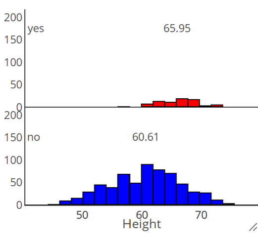
This tells us that removing height changes the se residuals (expect to increase) and the coefficient of smoker (if it’s now significant with a smaller residual standard error, then it increased). But by the coefficient of smoker changing, that tells us there is also a relationship between height and smoking status in this dataset.

Example R output with indicator coding.

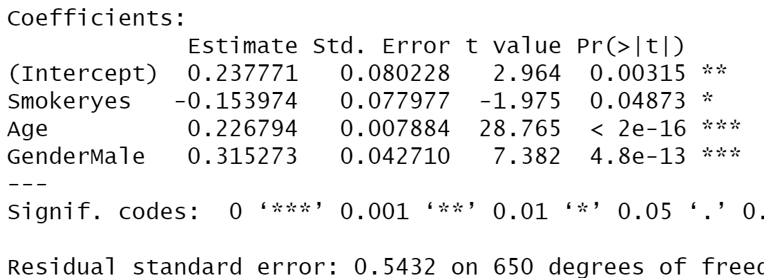
When we take out height, smoker because a proxy for taller (and older) people

3) Squid data

(a) Is there seasonality in the data?

We do see evidence in the boxplots that the median Testisweight varies noticeably across the months suggesting seasonality.

(b) Does the variability in the response appear to vary by month? Identify 3 months where you think our predictions of Testisweight will be most accurate. Least?

We also see evidence in the boxplots that the box widths differ noticeably across the months, suggesting unequal variances in the Testis weights among the different months. Months 7 and 8 has less variation (more accurate) and Months 9 and 10 seem the least accurate.

(c) If this model was fit with indicator coding and fMONTH = 1 as the reference group, is the coefficient of fMONTH2 positive or negative?

Month 2 is lower than Month 1 so the coefficient will be negative.

(d) If this model was fit with effect coding, is the coefficient of fMONTH2 positive or negative?

Month 2 is above average, so the coefficient will be positive.

(e) Continuing (d): If fMONTH1 is the missing category, will its coefficient be positive or negative?

Month 1 is above average, so the coefficient will be positive. Or if we had displayed all the other coefficients, we could sum them together and see the sum comes out negative.

But for addressing the unequal variance: We don't want to assume a "linear relationship" between the variability in the residuals and month number, so we will estimate the variance for each month. We can do that by finding the sample variance for each month.

(f) Which months do we want to 'downweight' in estimating the model?

The months with more variability, e.g., months 9 and 10.

(g) Conjecture what changes you would expect to see in the previous two graphs in this weighted regression model.

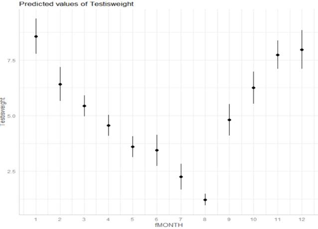
Now we are going to let the variances vary by month, so the graph of the fitted model would have much larger SEs for months 9 and 10, and smaller for months 7 and 8.

(h) How do you expect the residual standard error to change in the weighted regression model?

We expect months 7 and 8 to have pretty small values and then the other months will be multipliers for based on the larger month SDs. The small corresponds to a smaller residual standard error.

4) AirBnb

(a) Level 1 = AirBnB listing; Level 2 = neighborhood

(b) Level equations

Level 1:

Level 2:

and

(c) Which do you expect to be larger or ? Explain your reasoning.

Conceptually we might expect more variation in prices between listings in the same neighborhood but maybe less variation in the mean price listings across neighborhoods.

(d) Interpret the intercept coefficient in context.

The intercept ($25.35) is the predicted price for a listing for the entire house/department with 0 satisfaction rating in the average neighborhood.

(e) Interpret the coefficient of overall_satisfaction in context.

A one-point increase in the overall satisfaction rating, after adjusting for neighborhood and room type, predicts a $24.92 increase in the (average) price.

(f) Based on this output, is the type of room statistically significant? State the null and alternative hypothesis in terms of regression parameters, and clearly justify your answer.

Using the partial F-test from the ANOVA table, the p-value is very small because the F-statistic is very large (244.195)

(g) Consider the following two variables:

PctBlack would allow a more “granular” look at the relationship, the rate of decrease in predicted price with each additional percentage point, BUT, that relationship would need to be linear. Look at a graph before adding PctBlack into the model. If the relationship isn’t linear, then using the binary version could be an alternative. I am assuming that prices decreases with increasing percentage black in the neighborhood so predict a negative coefficient (including for the binary variable as 1 corresponds to the higher percentage).

(h) If HighBlack is added to the model how/if do you expect or to change? Explain your reasoning (for each).

This is a Level 2 variable so we don’t expect to change but do expect to decrease.

(i) Consider the first few observations of the first row of the variance-covariance matrix for the above model output

Where will the first zero value occur?

Depends how many observations there are in the first neighborhood. If that number is K, then K+1 through the 1561 columns of that first row will be zero, as those would all be other neighborhoods and we are assuming observations in different neighborhoods are not correlated.

(j) Here is the first row of the corresponding correlation matrix

Verify the value for 0.0861.

487.0952/(5657.442) = .086

(k) If I were to look at the first row of the corresponding correlation matrix for the null model, how do you think the second value will compare? (likely) Explain your reasoning.

Typically (but not always), the within-group correlation will be larger in the model that doesn’t explain any of the Level 1 and Level 2 variability.

5) Which model demonstrates more school-to-school variability in language scores?

On average, the slope coefficients are larger in magnitude for the modelling including IQ_verb. It’s counter intuitive, but in this case, after adjusting for IQ_verb, there is actually more school-to-school variation. The main cause is that within school and between school relationships are not consistent, schools with lower language scores tended to have higher IQ_verb scores, so after adjusting for IQ_verb, the “additional contribution” to match the school means is larger.

6) Consider this paragraph: The multilevel models we have considered up to this point control for clustering, and allow us to quantify the extent of dependency and to investigate whether the effects of level 1 variables vary across these clusters.

(a) I have underlined 3 components, explain in detail what each of these components means in the multilevel model.

Control for clustering: We have observations that fall into natural groups and we don’t want to treat the observations within the groups as independent, by including the “clustering variable” in the model, the other slope coefficients will be “adjusted” or “controlled” for that clustering variable (whether we treat it as fixed or random)

Quantify the extent of the dependency: The ICC measures how correlated are the observations in the same group

Whether the effects of level 1 variables vary across the clusters: random slopes

(b) The multilevel model referenced in the paragraph does not account for “contextual effects.” What is meant by that?

The ability to include Level 2 variables, variables explaining differences among the clusters. In particular, we can aggregate level one variables to be at Level 2 (e.g., group means). Being able to include these in the model, along with controlling for the individual groups, is another huge advantage of multilevel models.

7) Give a short rule in your own words describing when an interpretation of an estimated coefficient should “hold constant” another covariate or “set to 0” that covariate

We should hold variable 2 constant (which can include random effects) when we are interpreting the slope of variable 1.

We should put all explanatory variables (including the Level 2 random effects) at zero when interpreting an intercept. In a random intercepts (only) model, all the slopes are the same so you can say “in a particular school”

8) SAS output

(a) What is the patient level variance? (Clarify any assumptions you are making about the output/any clues you have.)

Because the first table is titled “covariance,” I’m assuming those are estimated variances rather than estimated standard deviations. The patient to patient variance is estimated to be = 73.7 mmHG² (within the same clincial center)

(b) What is the center level variance?

The center to center variance is estimated to be = 10.7 mmHG²

(c) What is an estimate of the ICC? Calculate and interpret.

10.7 / (10.7 + 73.6) approx 0.13. This represents the correlation btween two patients at the same clinic and that 13% of the variation in diastlic blood pressure is at the clinic level.

(d) What is the expected diastolic blood pressure for a randomly selected patient receiving treatment C at a center with average aggregate blood pressure scores?

90.97 mmHG, the intercept (no treatment C effect and no clinic effect because at the average center)

(e) What is the expected diastolic blood pressure for a randomly selected patient receiving treatment A at a center with aggregated blood pressure scores at the median?

Because we are assuming the clinic effects are normally distributed, with a center at the median, is again assumed to be zero. So 90.87 + 3.11 to include the effect of treatment A = 93.98 mmHG.

(f) What is the expected diastolic blood pressure for a randomly selected patient receiving treatment C at a center with aggregate blood pressure scores at the 16th percentile?

Now we want to assume the clinic effect is 1SD below zero where the random clinic effects are assumed to be normally distributed with mean zero and standard deviation = sqrt(10.67). So a clinic at the 16^th percentile is predicted to fall 3.27 below the average across all the clinics.

So 90.87 (intercept) + 0 (treatment C) – 3.27 (random effect for 16^th percentile) = 87.60 mmHG.

(g) What is the expected diastolic blood pressure for a randomly selected patient receiving treatment B at a center with aggregate blood pressure scores at the 97.5th percentile?

Now we want to assume the clinic effect is 2SD above zero = 2(3.27)

So 90.87 + 1.41 + 2(3.27) = 98.82 mmHG.

9) For a sample of 400 children from the National Longitudinal Survey of Youth, we have data on the child’s cognitive test score at age 3 (“ppvt”), the mother’s level of education, and the mother’s age at the time she gave birth.

Below are the graphs and output related to regressing the ppvt score on the mother’s age

For each assumption below, comment on whether you think it is met. Explain how you are deciding or what additional information you would need. If you think the assumption is violated, explain the nature of the violation.

(a) (2 pts) Linearity The Residuals vs. Fitted graph shows only minor curvature (the red smoother is almost flat) indicating that the linearity assumption is satisfied (removing the linear components leaves random scatter rather than a pattern)

(b) (2 pts) Equal variance The Scale-Location graph does show a slight downward trend (showing a gradual decrease in the overall magnitude of the residuals as shown a bit by fanning in in the Residuals vs. Fitted graph as well) but the largest SD does not appear to be more than twice the size of the smallest SD so I could consider this condition sufficiently met.

(c) (2 pts) Normality We would need a graph (histogram or normal probability plot) of the residuals

(d) (2 pts) Independence We were told this was a professional collected sample so if we consider it a random sample from the population of interest, with no repeat observations are even multiple children from the same family, then the independence condition is met. If they were cluster sampled from different neighborhoods, then we might have some concerns.

For same dataset, model

10) (a) (3 pts) Provide a one-sentence interpretation of the following output

predict(model4, newdata = data.frame(momage=30), interval = "prediction")

fit lwr upr

1 95.89836 56.38459 135.4121

I’m 95% confident that a single 30-year old mom will have a child with ppvt score between 56.4 and 135.4.

(b) (2 pts) Suppose instead we used interval = "confidence"

1. Identify one thing that will not change

The midpoint (“fit”) of the interval will not change.

2. Identify one thing that will change

The width of the interval will be much smaller because now it’s an interval for the population of pvt scores for all children with mom age = 30 years.