BRIEF SOLUTIONS TO INCLASS INVESTIGATIONS – Chapter 1
Last Updated January
1, 2014
Investigation 0
(a) Calls for
prediction
(b)-(f) Answers will vary but should see results vary from
student to student
(g) conduct more repetitions
(h) The proportion
bounces around for a while but then settles down around one value
(i)
Results will vary, should be close to 0.375
(j) Should be close
to 1-0.375 = 0.625
(k) 4
(l) 3, because one 3
mom/babies match, the fourth must as well
(m) Answers will
vary, should be close to 1
(n) The average
bounces around for a while but then settles down about one value
(o) 24
(p)
|
1234 = 4 |
1243 = 2 |
1324 = 2 |
1342 = 1 |
1423 = 1 |
1432 = 2 |
|
2134 = 2 |
2143 = 0 |
2314 = 1 |
2341 = 0 |
2413 = 0 |
2431 = 1 |
|
3124 = 1 |
3142 = 0 |
3214 = 2 |
3241 = 1 |
3412 = 0 |
3421 = 0 |
|
4123 = 0 |
4132 = 1 |
4213 = 1 |
4231 = 2 |
4312 = 0 |
4321 = 0 |
(q) 9
(r)
9/24 = 0.375
(s)
|
#matches |
0 |
1 |
2 |
3 |
4 |
|
probability |
9/24 |
8/24 |
6/24 |
0 |
1/24 |
(t) one, because these are all the possibilities
(u) 8/24 + 6/24 +
1/24 = 1- P(X = 0) = 1- 9/24 = 15/24
(v) E(X) = 9(9/24) +
1(8/24) + 2(6/24) + 4(1/24) = 1
(w) No, zero is the
most probable outcome. What is meant by “expected value” is the long-run
average outcome
(x) V(X) = (0-1)2(9/24)
+ 0 + (2-1)2(6/24) + 0 + (4-1)2/24 = 9/24 + 6/25 + 9/24 =
1
SD(X) = 1
Investigation 1.1
(a) 14/16 = 0.875
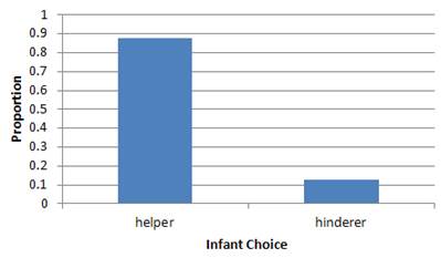
(b) Possible explanations
Infants’ selections are influenced by the behavior displayed in the videos
Random chance
Note: We are not considering the color, shape, or position of the object as the explanation for the infants’ choice as these factors were balanced in the design of the study.
(c) The “random chance alone” possibility means that each infant was equally likely to choose among the two toys. Otherwise, there are lots of possible probabilities at play.
(d) Yes, it is possible that we could get 14 choosing the helper even if the infants were choosing blindly between the two objects.
(e) These results will help us assess the variability in the outcomes of 16 infants “just by chance.” This will help us decide whether 14 is a typical outcome or an unusual outcome when we know for a fact that the “infants” choose equally (in the long run) between the two toys.
(f) Toss a coin 16 times, letting heads represent an infant choosing the helper.
(g) 8
(h) no, there will be variability across the sets of 16 tosses
(i)-(k) Results will vary by class, below is one possible set of results.
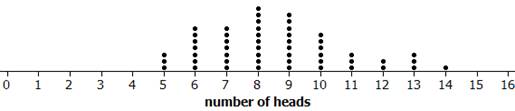
(l) 8 is the most frequent outcome, and results from 6-10 are pretty common.
(m) An outcome of 14 only happened once in these 51 trials, indicating 14 heads (choosing the helper) is a fairly surprising outcome under the null mode.
(n) Answers will vary.
(o) Answers will vary, e.g., 8, 5, 5, 9
(p) Delete this question
(q) center: 8
spread: roughly 2 to 14
shape: symmetric bell shape
(r) This is what we would see if we were to repeat the process 1000 times where we know it’s 50/50
(s) Example response:
Count: 4
Proportion: 4/1000 = 0.004
(t) No, and this proportion will vary from person to person by chance because we aren’t taking all possible samples
(u) Very surprising
(v) Yes because it is very unlikely for us to have seen results at least as extreme as what we observed (14 successes) under the assumption of 50-50 chance.
(w) No, p-value too small.
(x) Risky because we aren’t given any information about these infants other than their age. Although there also is no obvious reason to believe these infants would behave any differently on this issue than other infants.
Probability Exploration: Mathematical Model
(a) no, but pretty close
(b) ![]() (.5)14(1-.5)2
=
(.5)14(1-.5)2
= ![]() (.5)16 = 0.0018
(.5)16 = 0.0018
(c) ![]() (.5)15(1-.5)1
= 16*(.5)16 = 0.00024
(.5)15(1-.5)1
= 16*(.5)16 = 0.00024
![]() (.5)16(1-.5)0
= (.5)16 = 0.0000153
(.5)16(1-.5)0
= (.5)16 = 0.0000153
(d) .0018 + .00024 + .0000153 = .0021
Comparison: Should be pretty close to the simulation results.
More Technical Details
(a) (14(1) +
2(0))/16 = 14/16 = 0.875
(b) We would have a
stack of height 14 at one and a stack of height 2 at zero, mimicking the bar
graph.
(c) The two stacks
would be the same height, 0.50.
(d) These results
are less consistent, there is not a “clear majority”
in the outcomes.
(e) The distances
are -0.5 and 0.5.
(f) If we take the
absolute value of the distances, then the average of the 16 0.5 values is
16(.5)/16 = 0.5
(g) The distances
are (1-.875) = 0.125 and (.875-0) = .875.
The average is (14(.125) + 2(.875)) / 16 = 0.21875
(h) The 8/8 split
has a larger average deviation/less consistency/more variability.
Investigation 1.2
(a) If everyone is just guessing, then a binomial model is appropriate:
A student puts Tim’s name on the left or not (two outcomes)
There are n trials (your class size)
The probability of success is 0.5 for every trial.
Assuming the students are not interacting, we can assume their responses are independent.
(b) Null model: no facial prototyping/ random chance/ equally likely to put Tom on the left as Bob
(c) Flip a coin (once for each person in the study), record the number of heads up (successes), and repeat this process a large amount of times (1000). This will help tell us what we types of results we might see if everyone was picking at equally at random between the two names.
(d) Results will vary, the following is from a class where 32 out of 45
picked Tim as the “scruffier” looking individual.
(e) More people picked the left face as Tim, 32/45 picked Tim on the left (0.71)
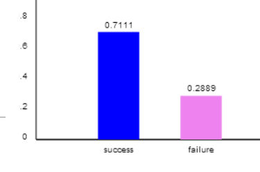
Vertical axis = proportion in each category
Success = picked Tim for face on left, Failure = picked Bob for face on left
(f) Observation units = 45 students
Variable = name on the left. Categorical, binary
Success= Tim on left. (This can also be Bob on the left, just make sure to be consistent with what you define as success)
(g) statistic: ![]() = 32/45 = 0.71
= 32/45 = 0.71
Parameter: π = probability that a student put Tim on the left (success) in general
(h) H0(null model): π = 0.5
(i) Ha: ![]() > 0.5
> 0.5
(j) X = number of students who chose Tim on the left. Want
to find P(X ≥32) where X is Binomial with n = 45 and ![]() = .5 (under the null
hypothesis)
= .5 (under the null
hypothesis)
(k) p-value = 0.0033
(l) 0.33% of “studies” based on 50-50 probability will have results at least as extreme as 32 Tims on the left.
(m) small (<.01). Statistically significant
(n) yes
Investigation 1.3
(a) obs units: cases or patients or heart transplantations
variable: whether or not the patient died within 30 days of the transplant
success: death within 30 days (could be either but this matches the 15%)
failure: survival
(b) Let ![]() represent the underlying
probability of death within 30 days of transplant at this hospital
represent the underlying
probability of death within 30 days of transplant at this hospital
(c) ![]() = .15
= .15
(d) ![]() > .15
> .15
(e) H0: ![]() = .15 (the death rate at
St. George’s is the same as the national average)
= .15 (the death rate at
St. George’s is the same as the national average)
Ha: ![]() > .15 (the death rate
at St. George’s is larger than the national average)
> .15 (the death rate
at St. George’s is larger than the national average)
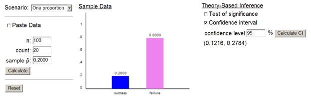
(f)![]() = 8/10 = 0.8
= 8/10 = 0.8
.8 > .15, so yes, the result is in the conjectured direction
(g) Want the p-value, which we find either through
simulation (with 10 trials and .15 as the probability of success) or using the
binomial distribution (with n = 10 and ![]() = .15). In both cases we
want to determine (estimate) P(X≥8)
= .15). In both cases we
want to determine (estimate) P(X≥8)
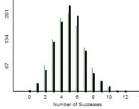
(h) Example results:
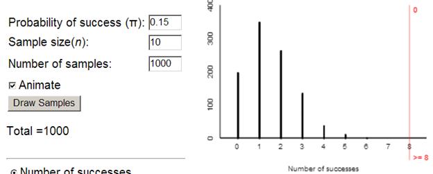
Shape is not symmetric (is actually “skewed to the right”)
(i) We see that we never get 8 or more successes so the p-value is approximately zero.
(j) zero
(R tells us the p-value equals 8.665 × 10⁻⁶)
(k) We have evidence to conclude ![]() > .15 (Ha).
We don’t think the higher mortality rate observed in these 10 cases happened
just by chance.
> .15 (Ha).
We don’t think the higher mortality rate observed in these 10 cases happened
just by chance.
(l) The null hypothesis would be H0: ![]() = 0.85 and the
alternative hypothesis would be Ha:
= 0.85 and the
alternative hypothesis would be Ha: ![]() < 0.85.
< 0.85.
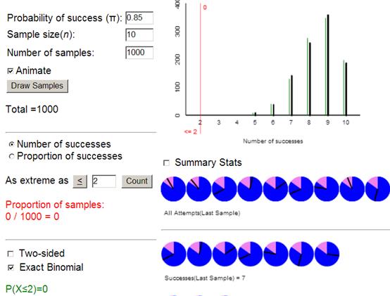
This turns out to be an equivalent analysis.
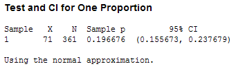
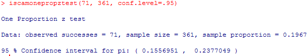
(m) ![]() = 71/361 = 0.197
= 71/361 = 0.197
This sample proportion is much closer to 0.15 but also based on a much later sample size.
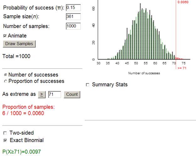
p-value » .01
(n) yes, small p-value. Reject H0
that ![]() = .15, convinced that
= .15, convinced that ![]() > .15
> .15
(o) a bit weaker (though still quite strong) demonstrated by the larger p-value.
Investigation 1.4
(a) obs units: couples (or kissing pairs)
variable: direction (left or right). Binary, we choose leaning to the right as success
statistic: ![]() = proportion of kissing couples that leaned to the right =
80/124 »
0.645
= proportion of kissing couples that leaned to the right =
80/124 »
0.645
parameter: ![]() = the overall chance or
probability that a kissing couple leans to the right.
= the overall chance or
probability that a kissing couple leans to the right.
(b) H0: ![]() = .75
= .75
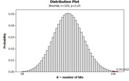
(c) Ha: ![]() ≠ .75
≠ .75
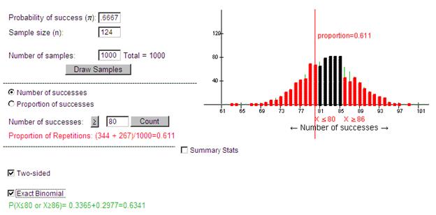
(d) .75(124) = 93
80 is 13 less than 93, so a reasonable value for the other side of the distribution would be 106 (13 greater than 93)
(e) P(X£80 or X ≥106) = P(X £80) + P(X ≥106) = .0093
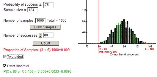
The applet used cut-off values of 80 and 106 as we anticipated. The two-sided p-value is around 0.009.
(f) yes. Small p-value.
(g)

This p-value is not small and we fail to reject the null hypothesis. It is plausible that the probability a kissing couple leans right is equal to 2/3.
Investigation 1.5
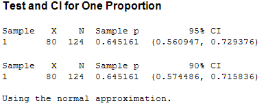
(a) our best single guess would be this value 80/124 » 0.645
(b) no, results can vary randomly from this value
(c) results may vary a bit from simulation to simulation but generally you should find this:

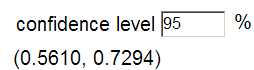
(d) This includes more values than the one based on the .05 criteria. This makes sense because with a higher confidence level we have more room for error.
![]()
(e) (0.55423, 0.72898)
(f) same midpoint but wider interval (.526, .752)
Investigation 1.6
(a) Let ![]() represent the player’s
now actual probability of getting a hit
represent the player’s
now actual probability of getting a hit
(b) H0: ![]() = 0.250 (he’s the same)
= 0.250 (he’s the same)
Ha: ![]() > 0.250 (he’s
genuinely improved)
> 0.250 (he’s
genuinely improved)
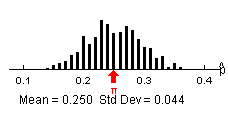
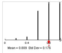
(c) Conjectures will vary: 20 is not a huge number, but he really has improved a lot
(d) The horizontal axis is the number of hits in 20 at-bats. The x-axis will range from 0 to 20, centered around 5, but we not that the distribution tails off pretty quickly after about 10.
The player would need probably 10 or more hits (answers may vary).
(e) Example results
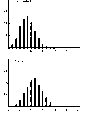
The two distributions overlap a lot. Not going to be likely to convince the manager that he’s not a .250 hitter.
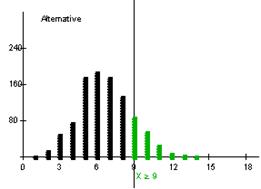
(f) Example results:
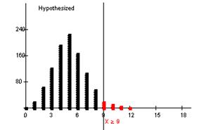
![]()
He would need to get 9 or more hits to be in the top 5% of the distribution for a .250 hitter.
(g) about 5% (3.7% above)
(h) A Type I error would mean the player has not improved but he does well enough in the sample of 20 at-bats to convince the manager that he has.
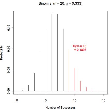
(i) Example results for the alternative distribution:
![]()
A little less than 20% chance that a .333 hitter will achieve 9 or more hits in 20 at-bats.
(j) A Type II error
means the player has improved but does not do well enough in his 20 at-bats to
convince the manager.
(k) Decision table:
|
|
Ho
true |
Ho
false |
|
Reject Ho |
type I error |
J |
|
Fail to reject Ho |
J |
type II error |
(l) Player would like to minimize the probability of a Type II error – of the manager missing his improvement
The manager would like to minimize the probability of a Type I error – incorrectly thinking the player has improved
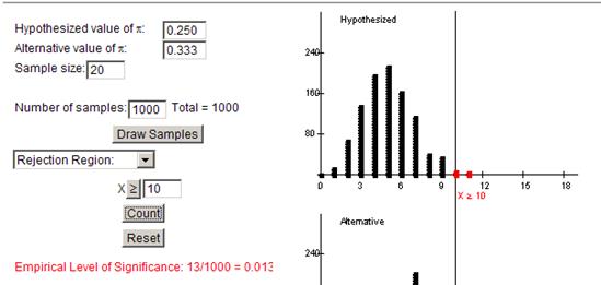
(m) He should require a higher standard of proof – more hits to convince him the player has improved, so changing the rejection region from 9 or more hits to 10 or more hits
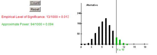
(n) In the simulation below, the probability of a type I error went down to about .01
(o) The power went down even more as well to less than .10.
(p) more at bats
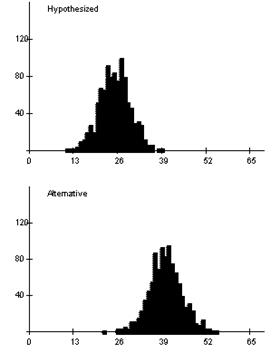
(q) For example:
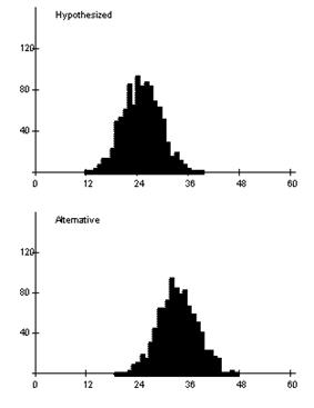
The distributions shift up to higher numbers but there is also less overlap between the distributions.
(r)
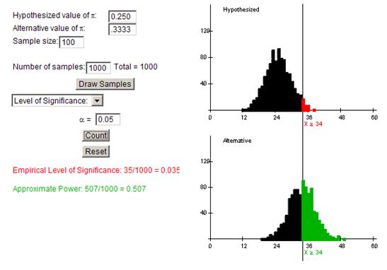
The new rejection region is 34 hits in 100 at bats or more.
(s) The power has risen above .50. This is much higher than the .18 we found before.
(t) This did help the player, the probability of him performing well enough to convince the manager he has improved is now much higher. This makes sense because the player really has improved and a larger sample size is more likely to reflect that and make it less likely that he has a “bad day” and performs below his true probability and looks like a .250 hitter. (Of course this is assuming the player doesn’t get tired out! J)
(u)
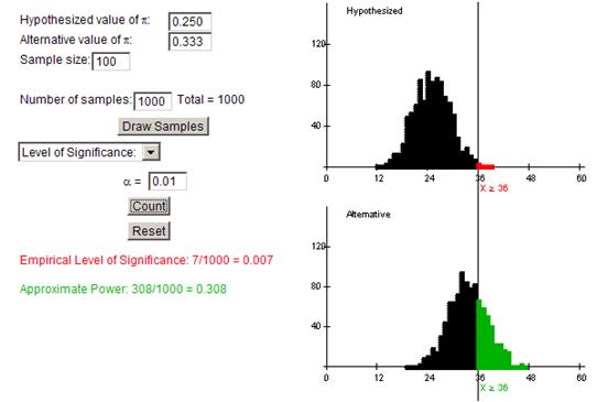
The new cut-off (rejection region) is 38 and the new empirical probability of a Type II error is .692 (1-.308). This did not help the player.
(v) Calls for conjecture.
(w)
![]()
The alternative distribution moves to the right (to center around .40 × 100 = 40).
There is even less overlap between the two distributions.
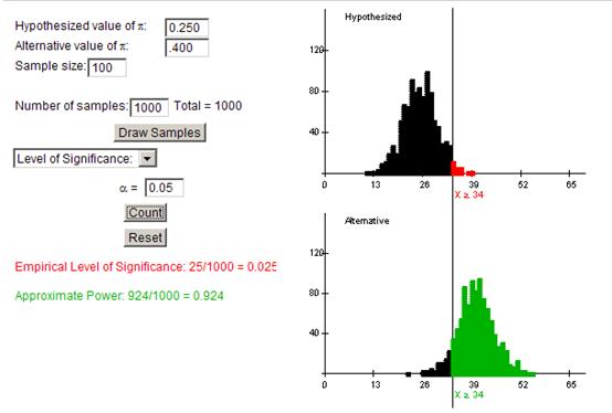
The cut-off value is 34. This is actually the same if we use a sample size of 100 and an alpha level of .05 with .333 as the alternative value, because it just depends on the .250 and level of significance.
The empirical power is .924, very high. It is much more likely for a .400 hitter to convince the manager he is not a .250 hitter than even for a .333 hitter.
(x) If P(Type I Error) decreases, then P(Type II Error) increases and vice versa. But the owner prefers small P(Type I Error) while the player prefers small P(Type II Error). The level of significance controls P(Type I Error). Increasing the sample size and increasing the alternative probability away from .250 both decreased P(Type II Error).
Probability
Exploration: Exact Binomial Power Calculations
(a) 1. Determine how well a .250 hitter would have to do to
have a p-value below .05 (the value specified by the manager as the level of
significance). That is, find k such that P(X > k) <
.05 where X ~ Bin(n=20,
![]() = .250)
= .250)
Using iscaminvbinom:
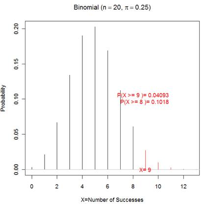
He needs at least 9 hits.
(Note, the actual probability of a type I error would be .04093)
(b) Determine how often a .333 hitter gets 9 or more hits,
P(X > 9) where X ~ Bin(n=20, ![]() = .333)
= .333)
Using iscambinomprob:
(c) See Demo
(d) Trial and error finds that an n of 189 has a rejection region of 58 and the probability that a .333 hitter gets at least 58 hits in 189 at bats is .8010.
Investigation 1.7
(a) Observation unit = Reese’s Pieces candy
Variable = color or whether or not color is orange
(b) No, we choose the candies at random so the results will vary
(c) This is a statistic because it is calculated about a sample
of data, ![]()
(d) Graphs will vary by student but should be a bar graph, with a bar for each color and height at the sample proportion for that color.
(e) Example class results:
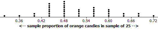
(f) Observational unit = sample of 25 candies (each sample is an observational unit)
Variable = proportion of orange in the sample, this is quantitative
(g) no
(h)The shape is roughly symmetric, with a center of around .50, the values range from .32 to .72.
(i) The actual probability that a
Reese’s Pieces candy is orange, ![]() , seems to be around .50
because that is where the
, seems to be around .50
because that is where the ![]() values are clustering.
values are clustering.
(j) You will probably obtain different![]() values, but if you add them up and divide, you
can find the average of the
values, but if you add them up and divide, you
can find the average of the ![]() values.
values.
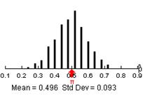
(k) The distribution should be pretty symmetric, centered around .5, mostly ranging from .3 to .7. This is the
distribution of sample proportions IF ![]() = .5, n= 25 and
the candies are drawn at random.
= .5, n= 25 and
the candies are drawn at random.
Example results:
(l) Calls for conjecture.
(m) The distribution “fills in” with the possible outcomes
falling closer together and closer to ![]() , meaning there is less spread
in the values. The values still center around .5, and
the shape is still roughly symmetric.
, meaning there is less spread
in the values. The values still center around .5, and
the shape is still roughly symmetric.
Example results:

(n) calls for conjecture
(o) Now the distribution will center around .25. The shape is still pretty symmetric and the values now range from .1 to .4
Example results:
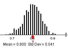
(p) Now the distribution centers around .80, it’s still symmetric, and the spread is from roughly .7 to .9.
Example results:
(q) The centers of all 3 distributions differ and the first distribution has a wider spread in values than the other two.
All three distributions have a symmetric shape.
(r)
|
|
Theoretical
mean of |
Theoretical SD of |
|
n
= 25, p = .5 |
.5 |
.10 |
|
n
= 100, p = .25 |
.25 |
.043 |
|
n = 100,
p = .80 |
.80 |
.04 |
These results very closely match those of the simulation
(s) mean = .80 and sd=.04
.8-.04 = .76
.8+.04 = .84
(t) Example results
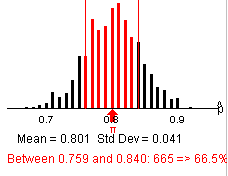
This percentage is in the ballpark of 68%.
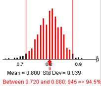
(u) Predicted by Empirical Rule: 95%
(v) The shape will no longer be symmetric and the spread will be larger (mean still around .80).
It would not be reasonable to model these outcomes with the normal distribution.
Note: Theoretical SD(![]() ) = sqrt(.8(.2)/5) = .179
which is still appropriate.
) = sqrt(.8(.2)/5) = .179
which is still appropriate.
(w) For each of the cases above, n ![]()
![]() and n
and n ![]() (1-
(1-![]() ) exceeded 10, and all three
cases showed symmetric distributions.
) exceeded 10, and all three
cases showed symmetric distributions.
(x) The probability of obtaining a sample proportion of .85
or higher is .11. Or about 11% of random samples from this process would
yield a ![]() value of .85 or higher.
value of .85 or higher.
Investigation 1.8
(a) H0: ![]() = .25 (randomly choosing among 4 images)
= .25 (randomly choosing among 4 images)
Ha: ![]() > .25 (ESP?)
> .25 (ESP?)
(b) ![]() = 106/329 » 0.322
= 106/329 » 0.322
(c) .25(329) = 82.5 > 10
.75(329) = 246.75 > 10 Yes!
(d) Approximately normal with mean equal to .25 and SD(![]() )=
)=![]() = 0.024
= 0.024
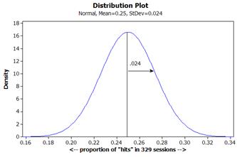
(e) shading under curve for 0.32 and to the right is too small to see.
(f) very small, less than 1%
(g) (.322 - .25)/.024 » 3.00
(h) Three standard deviations has an area to the right of about .3%/2 = 0.0015
(i) Normal approximation (mean = .25, SD = .024)
|
Minitab
|
R
|
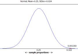
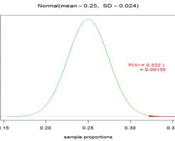
P(![]() > .322 when
> .322 when ![]() = .25 and n =
329)
= .25 and n =
329) ![]() .00135
.00135
(j) Exact Binomial (remember to use X = 106 as the observed result)
|
Minitab
|
R
|
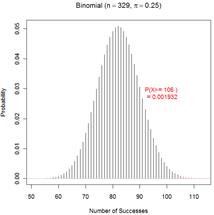
P(X > 106 when n = 329 and ![]() = .25) = .0019 (exact
probability)
= .25) = .0019 (exact
probability)
The normal model does appear to provide a reasonable approximation to the binomial probability in this case, as we expected.
(k) Interpretation: About .19% of random samples would have a result at least as extreme as the one observed (106 hits in 329 sessions) if all subjects are guessing at random among the 4 images (no ESP).
Conclusion: We have strong evidence that these subjects were not merely guessing among the 4 images but have a probability higher than .25 of identifying the correct image.
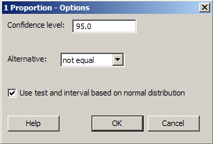
Investigation 1.9
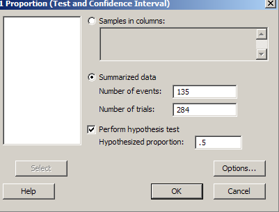
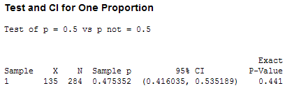
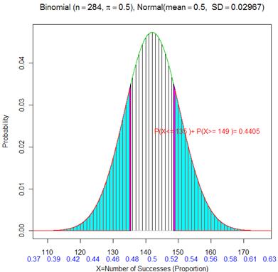
(a) Observational units=284 trick-or-treaters
Variable=whether chose candy or toy
Variable type: binary categorical
Possible outcomes: candy, toy
(b) Parameter=probability of choosing toy
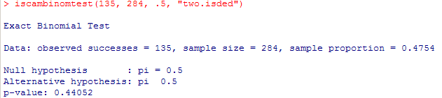
(c) Ho: ![]() = 0.5 (no general
preference for toys or candy)
= 0.5 (no general
preference for toys or candy)
Ha: ![]() ≠ 0.5 (either the
toys or the candy are favored
≠ 0.5 (either the
toys or the candy are favored
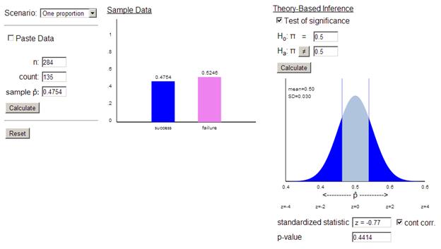
(d) Statistic: 135/284 = 0.475
(e) 284(.5) = 142 >10
284(1-.5)=142 >10, yes!
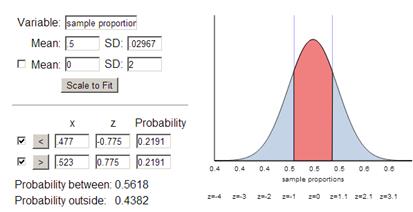
(f) What if distribution of ![]() ’s when
’s when ![]() =.5
=.5
Mean: .5(![]() =.5 in Ho)
=.5 in Ho)
SD(![]() ): sqrt(.5(.5)/284) = .0297
): sqrt(.5(.5)/284) = .0297
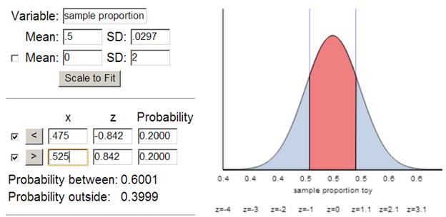
(g) z=![]() = -0.84
= -0.84
(h) negative because we’re below the mean
z(.525) = .84 (positive)
(i) no, less than one SD away
(j) about .40
|
Minitab
|
R
|
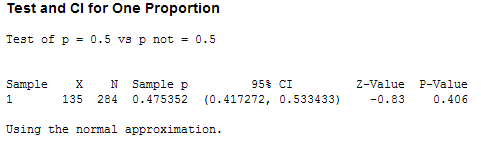
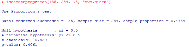
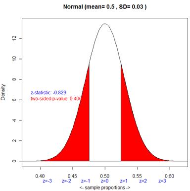
(k) 40% chance that at most 47.5% of kids or at least 52.5%
of kids will pick the toy if ![]() =.5, or about 40% of samples
will have
=.5, or about 40% of samples
will have ![]() < .475 or
< .475 or ![]() > .525 when there is no genuine overall
preference between candy and toys
> .525 when there is no genuine overall
preference between candy and toys
(l) p-value > .05 so fail to reject Ho. Not enough evidence of a genuine preference between candy and toy.
(m) probably happy with this- toy is viable alternative to candy
(n) no. Can’t know for certain, may not represent all kids, may be “special” toys & boring candy.
(o) 0.441
|
Minitab (not checking the “use normal”
box under Options) |
R
|
(p) P(X£135.5)
(q) P(X≥148.5)
(r) P(![]() < .477 or
< .477 or ![]() >
.523) ≈ .44
>
.523) ≈ .44
(s)
|
|
|
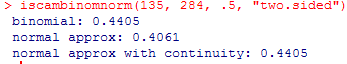
Note, there will be rounding discrepancies depending on how many
decimal places you use in the calculations.
Investigation 1.10
(a) n ![]() ≈ n ×
≈ n × ![]() (as we don’t have an estimate for
(as we don’t have an estimate for ![]() so use
so use ![]() ) = 124(.645)=80>10
) = 124(.645)=80>10
n(1- ![]() )=124(.355)=44>10 Yes!
)=124(.355)=44>10 Yes!
(b) approximately normal. mean? SD? (need ![]() )
)
(c) SE(![]() )=
)=![]()
(d) SE(![]() )=
)=![]() =0.043
=0.043
max plausible distance = 2*0.043 (95% of the time)
(e) ![]() should
fall within 2 standard deviations of the observed sample proportion
should
fall within 2 standard deviations of the observed sample proportion
So ![]() ≥ .645-2(.043)=.559,
≥ .645-2(.043)=.559, ![]() £ .645+2(.043)=.731
£ .645+2(.043)=.731
I’m 95% confident that the probability a kissing couple leans right is between (.559, .731)
(f) z = ± 1.96
(g) 1.645 < 1.96
only capturing the middle 90% so don’t have to extend as far from the middle
(h) midpoint: ![]() ; width: 2 × z*
; width: 2 × z*![]()
(i) if increase Confidence Level Þ increase z* Þ wider interval
if increase n Þ small width (n is in the denominator)
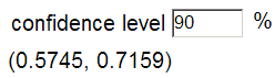
(j) If the confidence level is 90%, then use z* = 1.645
.645 – 1.645 × .043 = .5734
.645 + 1.645 × .043 .7157
I am 90% confident that between 57.3% and 71.6% of kissing couples turn to the right.
(k) midpoint = (.5734+.7157)/2 = .645
width = .7157 - .5734 = .142
2(1.645)(.043) = .142
(l)
|
Minitab
|
R |
|
Applet
|
|
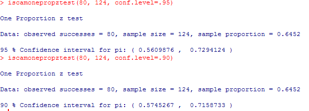
(m) The binomial confidence intervals are a bit longer (and even a bit more to the left)
(n) ![]()
![]() (put
in 2/3 as a reasonable guess for
(put
in 2/3 as a reasonable guess for ![]() , could also use the previous
, could also use the previous ![]() or .5)
or .5)
![]()
So we would need at least 949 couples.
(o)-(t) Results will vary from student to student but should
see that intervals change from sample to sample, but usually they are green
indicating that they correctly contained ![]() somewhere in the
interval. The long-run percentage of intervals that do capture
somewhere in the
interval. The long-run percentage of intervals that do capture ![]() should be close to 95%.
should be close to 95%.
(u)Yes, the coverage rate is close to the nominal 95% confidence level. We expected this because the normal approximation from the CLT should be valid here.
(v) The intervals shorten, and the coverage rate dips to 90%.
(w) The intervals shorten, but the coverage rate stays around 90%.
(x) .95
(y) There is nothing “random” here, once the interval
is calculated, it either captures ![]() or it doesn’t. The
probability statement needs to be about the method, before you calculate
the interval.
or it doesn’t. The
probability statement needs to be about the method, before you calculate
the interval.
Investigation 1.11
(a) .8 + 1.96 sqrt(.8(.2)/10) => (0.552, 1.05)
But not passing the technical conditions necessary for this interval procedure to be valid.
(b) The coverage rate is not close to 95%, but closer to 80%.
(c) Sample size is too small for the binomial distribution to be approximated by the normal distribution.
(d) Now the coverage rate is much closer to 95%.
(e) The midpoints shift towards .5, this moves the midpoints off of zero and gives all intervals a positive length.
(f) 10/14 » 0.714
.714 + 1.96 sqrt(.714(1-.714)/14) = .714 + .2367 => (0.477, 0.951)
I am 95% confident that the underlying mortality rate at St. George’s Hospital is between .477 and .951.
(g) wald: (0.156, 0.238)
adj wald: (.160, .241)
|
Minitab
(Wald)
(Adjusted
Wald)
|
R
|
Investigation 1.12
(a) choices will vary
(b) length of word: quantitative
whether or not contains more than 4 letters: categorical
(c) Answers will vary
(d) Results will vary
obs units: words
Variable = length of word
(e) statistic, from sample of ten. ![]()
(f) parameter, about entire
population. ![]()
(g) no
(h) Example results:
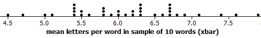
Obs units: sample of 10 words.
Variable: mean number of letters per word in the sample
Symmetric, center 6.5, spread 4.5 to 8. (approximate)
(i) above (everyone in this class produced a sample mean that exceeded the population mean)
(j) people tend to over represent larger words.
(k) will still have a higher probability of selecting the longer words because they take up more space
(l) randomly!
(m) Results will vary
(n) Example results
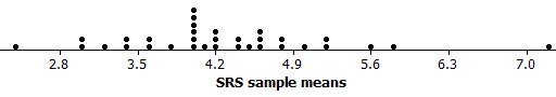
This graph is centered much closer to 4.29, though maybe a bit more spread out.
(o) no; no; they now cluster around the population mean
(p) about half
This sampling method is unbiased because the average of our results over several samples is close to the population mean.
(q) Yes, even with the smaller sample size, the improved selection method reduced the bias.
Investigation 1.13
a) population: all US voters
sample: 2.4 million respondents
sampling frame: telephone books and vehicle registration lists
parameter: ![]() = proportion of all US
voters for Alf Landon
= proportion of all US
voters for Alf Landon
statistic: ![]() = .57
= .57
b) 1. Oversampled republicans because Republicans tended to have more money for cars, phones in 1936. (bad sampling frame)
2. voluntary response bias. Hear from unhappy people
Investigation 1.14
(b) Categorical, ![]() = .47
= .47
(c)-(f) results will vary, but
should see ![]() values that vary from sample to sample
values that vary from sample to sample
(g) Yes because the average of the 500 ![]() values is close to
values is close to ![]() = .47
= .47
(h) Example results
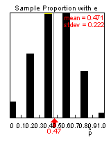
Mean: .471, Standard deviation .222
(i) ![]() = .47
= .47
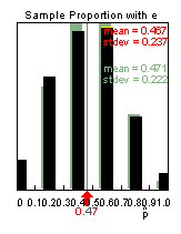
(j) mean, standard deviation, and shape are all pretty much the same as in (h) and (i)
(k) mean, standard deviation, and shape are all pretty much the same as in (j)
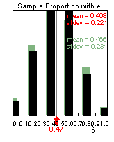
(l) Theoretical mean = .47 (![]() ), Theoretical standard
deviation = sqrt(.47(.53)/5) = .223
), Theoretical standard
deviation = sqrt(.47(.53)/5) = .223
These are very close to the results displayed in the applet as we would expect.
(m) No, because the sample size (n = 5) is small, so we can’t assume the normal approximation would be valid (there is too much separation between the possible outcomes).
Investigation 1.15
(a) The observational units are the freshmen; the response variable is whether they planned to vote for Kerry or Bush (categorical and binary).
(b) The sample is the 30 respondents, the population is the 705 first-years on campus, and the sampling frame is the list of residence halls, and then the rooms within the residence halls.
(c) Not every possible sample of 30 respondents is equally likely to occur because all samples will only select freshmen from within the same dorm. This was a “multistage systematic sampling plan.” It is still considered a random sample because they randomly chose dorms, then rooms within dorms (every 7th room). This method should be unbiased but because they only selected one dorm they do need to be cautious that students in that dorm do not feel tremendously different on this issue than students in the other dorms (which seems like a plausible belief).
(d) The surveys were anonymous and confidential and the names of the candidates were rotated.
(e)
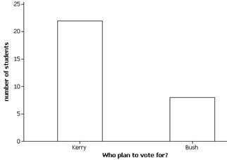
The sample reveals that most students (73%) planned to vote for Kerry.
(f)
The proportion of all freshmen at this school that were
planning to vote for Kerry (![]() )
)
(g) The observations are not independent. Say we select a success first. Then the probability of success will now be different because both the number of successes and the number of observations in the population will have changed.
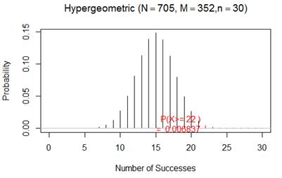
(h) Let X count how many of the 30 respondents choose Kerry, where the sample comes from a population with 352 successes (Kerry voters) and 705 – 352 = 353 failures (Bush voters). Then we can model X’s distribution as hypergeometric with N = 705, M = 352, and n = 30. The probability of finding 22 or more successes in such a sample is only about .0068. Therefore, we would consider this observation surprising to arise by chance alone from such a population. This indicates that about .68% of random samples would yield a result this extreme if Kerry and Bush were equally preferred in the population. This provides strong evidence that the claim about the population is incorrect.
![]()
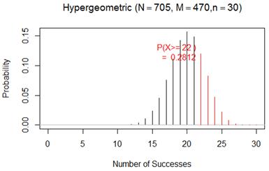
(i) If instead we assume 2/3 of the population planned to vote for Kerry, then we need to use the hypergeometric with N = 705, M = 470 (2/3 of 705), and n = 30. Now P(X > 22) ≈ .281. This indicates that about 28% of random samples would yield a result this extreme if two-thirds of the population planned to vote for Kerry. We would not consider an outcome of 22 to be surprising if 2/3 of the population were “successes” (planning to vote for Kerry).
(j) The population size of 705 is more than 20 times the sample size of 30, so this approximation is considered valid. Thus, the population size doesn’t matter, and we can consider the probability of success to be essentially constant for every observation in the sample. As shown below, the binomial p-value is quite similar.
![]()
Investigation 1.16
(a) population: all US teens
parameter: proportion of all US
teens that have at least some level of hearing loss.(![]() )
)
(b) Ho: ![]() = .20 (1 in 5 U.S. teens
has hearing loss)
= .20 (1 in 5 U.S. teens
has hearing loss)
Ha: ![]() ≠ 0.20 (headline
is not accurate)
≠ 0.20 (headline
is not accurate)
(c) Now have two things to consider
Sample size: n = 1771, ![]() = .2 .2(1771) >10 and
.8(1771) > 10
= .2 .2(1771) >10 and
.8(1771) > 10
Population size: N > 20(1771) yes, are more than 21 million American teens
(d) z= (.188-.20)/sqrt(.20(.80)/1771) = -1.26
p-value=0.2068
(e) no, .2068 > .05, fail to reject Ho.
These data do not provide convincing evidence that ![]() ≠ 0.2.
≠ 0.2.
Reasoning: A ![]() of .188 or more extreme happens in 20% of
samples from a population with
of .188 or more extreme happens in 20% of
samples from a population with ![]() = 0.2
= 0.2
(f) (.17, .206) I’m 95% confident that 17% to 20.6% of all
US teens have hearing loss. This is consistent with our test because 0.2
(hypothesized value of ![]() ) is in this interval –
plausible value for
) is in this interval –
plausible value for ![]() .
.
If asked to also interpret “confidence level”: By 95%
confident I mean in the long run 95% of intervals contain ![]() … (this method works 95% of
the time)
… (this method works 95% of
the time)
(g) yes, trust NHANES claims national representative sample…
Investigation 1.16
(a) observational units = American households
Variable = whether
or not there is a cat in the household
(b) statistic, ![]() , because it is computed on the sample
, because it is computed on the sample
(c) Let π
represent the proportion of all American households with a cat
H0:
π = 1/3 (population proportion equals one-third)
Ha: π ![]() 1/3 (differs from one-third)
1/3 (differs from one-third)
Because the sample size is large and because the population size is large,
I will use a z-test.
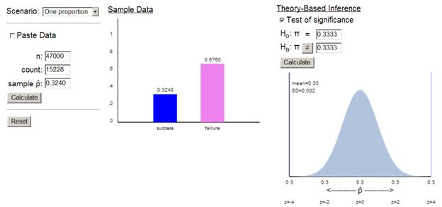
With such a
large test statistic and such a small p-value, we will soundly reject the null
hypothesis and conclude that we have convincing evidence at the .01 level
(.0000 < .01) that the proportion of American households with a cat differs
from 1/3.
(d) The p-value
is so small because the sample size is so large.
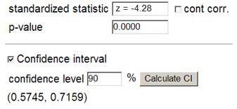
(e) We are 99%
confident that between 31.8% and 33.0% of American households own a pet cat.
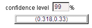
(f) This is
consistent because the confidence interval does not include .3333.
(g) Yes the
evidence is very strong because the p-value is small.
(h) No, the
confidence interval is very close to .3333, so even though we have strong
evidence π differs form one-third, the confidence interval shows us that
it’s not different by a lot, that is, not in a practical sense.
Investigation 1.17
(a)
(b) No, we know
the population proportion of females to be much closer to .50.
(c) This was a
bad sampling method (bad sampling frame) and can’t be saved by our formulas.
(d) No, if
π is the proportion of the 2013 senate that were women, then π = .20
case closed. We would have done a census
and have no justification for the inference.