BRIEF SOLUTIONS TO INCLASS INVESTIGATIONS – Chapter 4

Last Updated August 22, 2013

Investigation 4.1: Dr. Spock’s Trial

(a)

	Judge 1	Judge 2	Judge 3	Judge 4	Judge 5	Judge 6	Judge 7
Proportion of women	.336	.270	.291	.341	.270	.270	.144

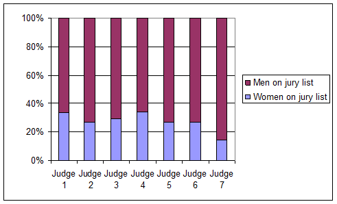
There is some variability in the proportion of women seen by each judge. Judge 7 in particular has a much lower percentage of women on his jury lists.

(b) [Let p_i represent the probability of a female juror for judge i.]

H₀: p₁ = p₂= p₃= p₄= p₅= p₆= p₇ (all seven judges have the sample probability of a female on the jury list)

H_a: at least one judge has a different probability

(d) Judge 1 saw 354 jurors so we would expect .261(354) = 92.39 females out of 354 and 261.61 men.

(e) Judge 2 saw 730 jurors so we would expect .261(730) = 190.53 women and 538.47 men.

(f) The expected counts are given below in red.

	Judge 1	Judge 2	Judge 3	Judge 4	Judge 5	Judge 6	Judge 7
Women on jury list	119 92.39	197 190.53	118 105.71	77 58.99	30 28.97	149 144.07	86 155.82
Men on jury list	235 261.61	533 538.47	287 299.30	149 167.01	81 82.03	403 407.93	511 441.18
Total	354	730	405	226	111	552	597

(g) The observed counts and the expected counts differ, however this could be due to random chance.

(h) Suggestions will vary.

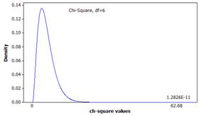
(i) The sum is approximately 62.68

(j) This calculation will result in larger values when the null hypothesis is false and smaller values when the null hypothesis is true, but it will always be nonnegative.

(k) We want to take a random sample of results for each judge (with varying sample sizes) but all with the same probability of a female juror. Once we have the results for each judge, we calculate the chi-square test statistic. We repeat this many times to see the pattern in these simulated chi-square values that arise just from the random sampling process alone. This will allow us to determine whether our observed chi-square result is surprising when the null hypothesis is true.

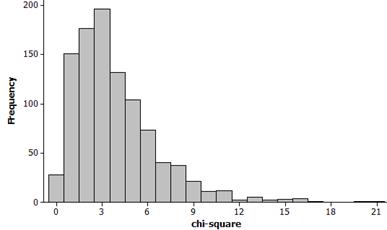
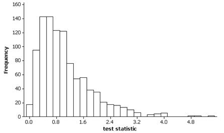
(l)-(m) Example empirical sampling distribution (1000 observations):

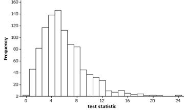
This distribution is skewed to the right. The mean should be around 6.

(n) None of the simulated sums is anywhere near 62.68.

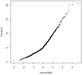
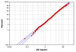
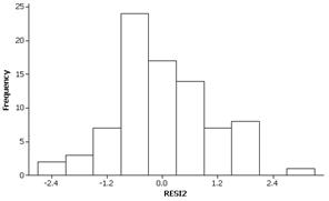
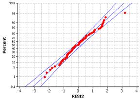
(o) There is strong evidence that these observations do not follow a normal distribution.

Example probability plot from R:

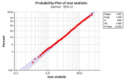
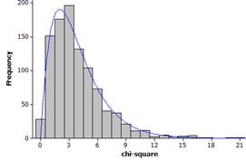
(p)-(q) The distribution should seem reasonably well modeled by a gamma distribution with parameters approximately 3 and 2 (a chi-square distribution with df = 6).

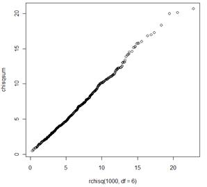
(r)

This indicates a p-value of approximately zero.

The p-value from the chi-square distribution is similar to the p-value from the empirical sampling distribution.

(s) The contributions from Judge 7’s cells are the largest.

(t) The observed number of women is less than expected and the observed number of men is larger than expected. This provides evidence that the proportion of women for Judge 7 is less than expected, even more so than any of the other judges.

(u) Judge 7.

Investigation 4.2: Near-Sightedness and Night Lights (cont.)

(a) far-sighted = 91/479: .190, normal: 251/479 » .524, near-sighted: 137/479 » .286

(b) There were 172 children in the darkness condition, so we expect 172(.19) and 172(.524) and 172(.286) or 32.68, 90.13, 49.19 in these 3 conditions.

(c) The proportional breakdown would be the same in all 3 groups if there was no association between eye condition and lighting level.

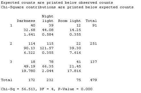
(d) Expected counts:

	Darkness	Night light	Room light	Total
Hyperopia	(40) 32.68	(39) 44.08	(12) 14.25	91
Emmetropia	(114) 90.13	(115) 121.57	(22) 39.30	251
Myopia	(18) 49.19	(78) 66.35	(41) 21.45	137
	172	232	75	479

(e) They are not all the same but the observed differences between the observed and expected counts could be due to random chance (e.g., the sampling process)

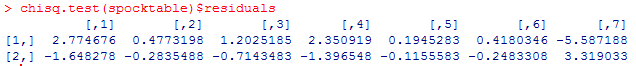
(f)

(g) The darkness/myopia cell and the room light/myopia cell have the largest contributions. We observed a smaller rate of myopia in the darkness group and a higher rate of myopia in the room light group than we would have expected if there was no differences among the lighting groups.

Technology Exploration: Randomization Test for Chi-square Statistic

(h) We could randomly reassign the response variable outcomes (eyesight condition) to the explanatory variable groups (lighting condition) and recalculate the chi-square statistic for each re-randomization. Then see how often we find a chi-square statistic at least as large as 56.513 just from this random assignment process (this assumes every child’s eye condition remains the same regardless of which lighting group they were in).

(i) Example simulation results

Possible R code

mychisq=0

for (i in 1:1000){

newrefraction=sample(refraction)

mychisq[i]=chisq.test(table(newrefraction, light))$statistic

}

(j) This does appear to follow a chi-square distribution

(k) The simulated p-value is less than 1 in 1000.

(l) Converting the simulated chi-square statistics into p-values or adding this command to the R code:

mypvalue[i]=chisq.test(table(newrefraction,light))$p.value

Example results:

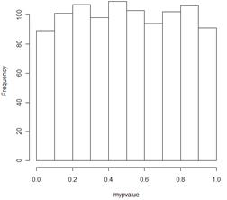
We find a uniform distribution between zero and one. This is what we would expect under the null hypothesis.

Investigation 4.3: Newspaper Credibility Decline

(a) The rotation guards against confounding variables such as fatigue that could play into later questions of the survey. We don’t want more negative ratings of later organizations just because they came towards the end of the survey.

(b) Two-way table:

	2002	1998
4	200	265	465
3	391	353	744
2	251	235	486
1	90	69	159
	932	922

H_a: There is at least one difference between the distributions.

The expected cell counts (see below) are all above 5 and we have independent random samples from 2002 and 1998.

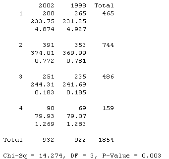
We have strong evidence (p-value = .003) to reject the null hypothesis and conclude that the population distributions did differ.

(d) H₀: p₉₈ = p₀₂vs. H_a: p₉₈ ≠ p₀₂

The expected cell counts are all above 5 (see below) and we have independent random samples from 1998 and 2002.

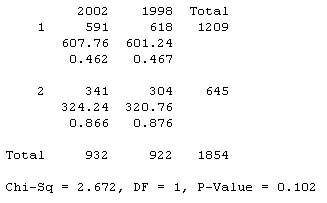
We fail to reject the null hypothesis. There is not convincing evidence that the population proportion who would rate their local paper as largely believable differed in 1998 and 2002.

(e) The test statistic we found before (z = -1.63) is smaller than the chi-squared value but the p-values are identical. In fact, squaring the z test statistic value gives the chi-square test statistic value.

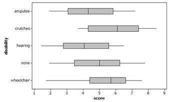
Investigation 4.4: Disability Discrimination

(a) The observational units are undergraduate students and the explanatory variable is the type of disability, the response variable is the rating of candidate’s qualifications. This is an experiment as the undergraduate students were randomly assigned to view one of the types of disabilities.

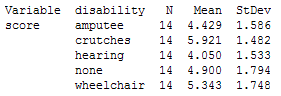
(b) Sample size, sample standard deviation

H₀: m_amp = m_crutch = m_hear = m_none = m_wheel

H_a: at least one of the m’s differs from the rest.

(d) Type I Error = thinking there is a difference in the effect of the disability types when there is not.

Type II Error = thinking there is a not a difference in the effect of the disability types when there is.

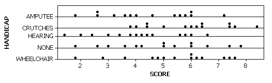
(e) The distributions appear similar in shape and center but have different amounts of variability within the groups. Graph B shows stronger evidence that the 5 samples did not all have the same overall mean.

(f)

There is some evidence of a difference in the average rating score given to the 5 different disability types.

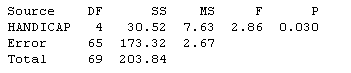
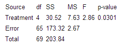
(g) The overall mean is 4.929.

(h) variance = .545

(i) Yes because the sample sizes are all equal.

(j) 14(.545) = 7.63

(k) average variance = (1.586² + 1.482² + 1.533² + 1.794² + 1.748²)/5 = 13.3357/5 = 2.67

(l) Our probability model is to consider the response ratings to be randomly assigned to the 5 treatment groups, so we expect similar variability in the 5 groups. This is confirmed by our observations from the numerical and graphical summaries of the results.

(m) 7.63/2.67 = 2.86

(n) Smallest value is zero which would result if there was no between group variation. There is no upper bound on the value this ratio can assume.

(o) This ratio will be large when the null hypothesis is false and small when it is true (but always nonnegative). In fact, when Ho is true, the ratio should be approximately one.

(p) We would put the 70 rating scores on index cards and then randomly assign 14 cards to 5 different groups and see what value of the test statistic we get for each randomization.

(q) Example empirical sampling distribution.

Possible R code:

myf=0

for (i in 1:1000){

newscore=sample(score)

means=tapply(newscore, dis, mean)

sds=tapply(newscore, dis, sd)

mst=sum(14*(means-mean(newscore))^2)/4

mse=sum((13)*sds*sds)/65

myf[i]=mst/mse

}

The empirical sampling distribution should be skewed to the right with mean about 1.

(r) Approximate p-value will be approximately .03 giving sufficient evidence to reject the null hypothesis at the 5% level.

(s)

(t)

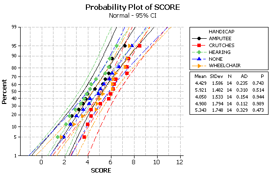
There is no evidence of nonnormality and the ratio of the largest to smallest sample standard deviation (1.794/1.482) is less than 2.

(u) There is moderate evidence that these average qualification ratings differ more than we would expect from the randomization process alone. There is at least one disability that has a different effect on the qualification ratings than the other disabilities. The ANOVA procedure appears valid since the observed treatment group distributions look reasonably normal and treatment group standard deviations are also similar.

Applet Exploration: Randomization Test for ANOVA

(a) H₀: no association between type of disability and rating

(b)

Group	None	Amputee	Crutches	Hearing	Wheelchair
Mean	4.900	4.429	5.921	4.050	5.343

(d) C(5,2) = 10 pairs

(e) So the positive and negative differences don’t cancel each other out

(f) MAD » 0.931

(g) results should match

(h) Answers will vary

(i) The results will vary from shuffle to shuffle

(j) Example results:

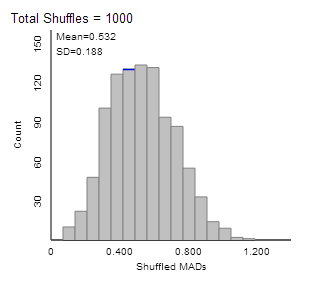
The distribution will have a slight skew to the right.

(k) the distribution is not centered at zero because the MAD statistic only takes on positive values.

(l) 0.931 or larger

(m) Example results:

(n) Example results:

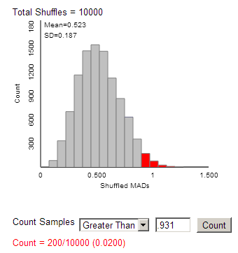
(o) 0.31 or larger assuming that the null hypothesis (no association) is true

(p) From the small p-value, we have strong evidence that there is a genuine associaiton between type of disability and employment rating.

(q) The F-test is more likely to find a statistically signficicant result when the null hypothesis is false.

(r) Observed F-statistic = 2.86

(s) Example results

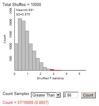
(t) The empirical p-value is smaller than the ANOVA table’s p-value.

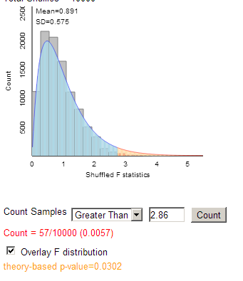
We see that the F distribution has a little bit heavier tail than our simulated null distribution.

(u) The p-values are all small and compared to 0.05, all lead us to reject the null hypothesis of no association. The evidence is strongest when looking at the simulated distribution of F-statistics.

Investigation 4.5: Restaurant Spending and Music

(a) weighted mean = [120(24.13) + 142(21.91) + 131(21.70)]/(120+142+131) = 22.52 (this is in the “middle” of the 3 observed averages).

Pooled variance = [119(2.243²)+141(2.627²)+130(3.332²)]/(119+141+130) = 7.73

Pooled std dev = sqrt(7.73) = 2.78 (this is in the “middle” of the observed standard deviations)

(b) H₀: the true treatment means (m_class = m_pop = m_none) are all equal

H_a: at least one true treatment mean differs

F = 226/7.73 = 29.2

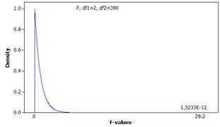
The p-value is approximately zero.

(d) We would need to be able to verify the technical conditions (in fact, there is an issue here in that the treatments were assigned to the evenings and not the individual dinners).

Applet Exploration: Exploring ANOVA

(e) Results will vary.

(f) Results will vary from sample to sample by chance.

(g) It will be possible to obtain a p-value below .05, but should happen less than 5% of the time (by chance alone).

(h) Now all the p-values should be quite small. We should have more evidence against the null hypothesis in this case as it is indeed false.

(i) The p-values tend to be larger, there will be less evidence against the null hypothesis from the smaller sample sizes (more variability due to chance).

(j) Larger values of s lead to larger p-values. This makes sense since larger values of s correspond to more variability in the treatment groups, making it harder to detect differences between the groups.

(k) The p-value will continue to get smaller since it will be easier to detect a difference when the size of the true difference is larger.

Investigation 4.6: Cat Jumping

(a) The observational units are the 18 cats and the primary response variable is takeoff velocity which is quantitative.

(b) Minitab output:

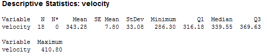
The distribution is pretty symmetric or skewed to the left a bit apart from an outlier in the 420 bin. Most cats had a velocity around 320-380 cm/sec but one was as small as 286.30 cm/sec and the high outlier was at 410.80 cm/sec.

Note: 300 cm/sec corresponds to about 6.7 miles per hour.

(d) Heavier cats might tend to have lower velocities.

(e) Minitab output

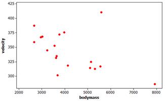
Overall, heavier cats tend to have lower velocity (though one of the heaviest cats had the largest velocity).

(f) ID: C

This cat has a much larger velocity than we would expect overall and for its weight.

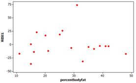
(g) Minitab output:

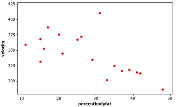
This also appears to be an overall trend of cats with higher body fat percentages having lower velocities on average, except for our same outlier.

(h) conjectures will vary.

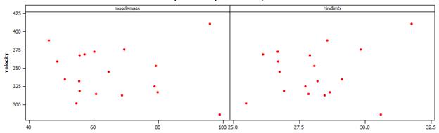
Muscle mass doesn’t appear to have as clear of a pattern but more muscle mass tends to have lower velocities.

Larger hind limb lengths tend to have larger velocities.

(i) Minitab output:

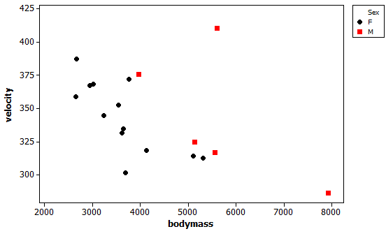
There are only 5 males but they tend to be heavier than the females. When the body mass is similar the velocities are similar though a little higher for males. The larger outlier is a male and there is also a very large male in terms of body mass.

Investigation 4.7: Drive for Show, Putt for Dough

(a) Negative, golfers that hit further will tend to be the same golfers with lower scores.

(b) Positive, golfers that hit more putts will tend to be the same golfers with higher scores.

(c)

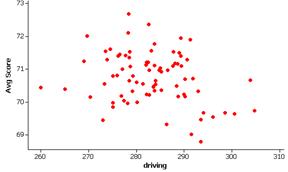
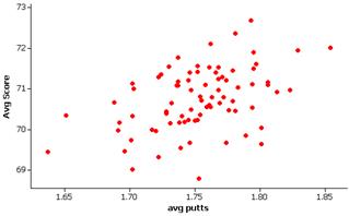
The relationship between average score and driving distance does appear to be negative. The relationship between average score and average putts appears positive and to be stronger than the first relationship.

(d) average score vs. average putts has more points in quadrants I and III

average score vs. driving has more points in quadrants II and IV

There appear to be fewer “unaligned points” in the average score vs. average putts graph.

(e) no measurement units

(f) the points will have random scatter, observations with below average x values will have both below and above average y values, observations with above average x values will have both below and above average y values.

(g) 1

(h) no, involves means, standard deviations, and squared terms, all of which should contribute to it not being resistant to outliers.

(i) rankings may vary

(j)

Strong neg	Medium neg	Weak neg	No association	Weak pos	Medium pos	Strong pos
-.835	-.715	-.336	-.013	.356	.654	.884

(k) smallest in absolute value: 0, largest in absolute value: 1

(l) r will be negative when the association is negative and positive if the association is positive

(m) no (linear) association

(n) perfect linear relationship

(o) scoring average and average putts which does support the cliché that putting is more related to overall scoring.

Applet Exploration: Correlation Guessing Game

Results will vary

(g) one (perfect linear relationship: guess = actual)

(h) one (perfect linear relationship: guess = actual + .2)

(i) No, as (h) showed, every guess could be wrong but still lead to an r of one.

Investigation 4.8: Height and Foot Size

(a) The observational units are the students, the explanatory variable is the person’s foot length and the response variable is the person’s height.

(b) The mean height of the 20 students: 67.75 inches

(d)

74	66	77	67	56	65	64	70	62	67
6.25	-1.75	9.25	-.75	-11.75	-2.75	-3.75	2.25	-5.57	-.75
66	64	69	73	74	70	65	72	71	63
-1.75	-3.75	1.25	5.25	6.25	2.25	-2.75	4.25	3.25	-4.75

We overestimated 11 times and underestimated 9 times.

(e) The residual is positive if the observation is above the fitted value and negative if the observation is below the fitted value.

(f) We could sum all the residuals as a measure of “total prediction error”

(g) The sum is zero

(h) S(y_i – ) =Sy_i – S = Sy_i – n = Sy_i – Sy_i = 0

(i) Could consider sum of squared residuals, sum of absolute residuals.

(j) Taking the derivative of S(m) = S(y_i – m)² and setting equal to zero

= (-2)S(y_i – m) = 0 and solving for m

= (-2)Sy_i + 2nm) = 0

2nm = 2Sy_i

So m = Sy_i/n, the sample mean.

Therefore, using the sample mean as our estimate for the variable will minimize the sum of the squared residuals, giving us the “best” prediction.

(k) There is a fairly strong (r = 0.711), positive, linear association between height and footlength. As expected, people with larger (above average) feet tend to also be taller (above average height).

(l)-(m) Lines will vary.

(n) Suggestions will vary.

(o) The best (smallest) SAE will vary.

(p) The smallest SSE will vary.

(q) Equation and resulting SSE values will vary.

(r) equation: = 38.302 + 1.033 foot size

SSE = 235

No should have been able to obtain a smaller SSE value.

(s) Taking the derivative…

(t) derivative with respect to b₀: S(-2)(y_i – b₀ – b₁x_i)

derivative with respect to b₁: S(-2x_i)(y_i – b₀ – b₁x_i)

(u) Setting to zero

Sy_i –b₁Sx_i = nb₀b₀ = Sy_i/n –b₁Sx_i/n

Sx_iy_i –b₁Sx_i² = b₀Sx_ib₁ = [Sx_iy_i- b₀Sx_i]/Sx_i²

(v) b₁ = .711(5.00/3.45) = 1.03

b₀ = 67.75 – 1.03(28.5) = 38.4

predicted height = 38.4 + 1.03 footlength

Note: Will be lots of rounding discrepancies.

(w) if footlength= 28cm, we predict a height of 38.4 + 1.03(28) = 67.24 inches

if footlength= 29 cm, we predict 38.4 + 1.03(29) = 68.27 inches

difference = 68.27 – 67.24 = 1.03 which is the same as the slope of the regression line

(x) The slope is the predicted difference in height for foot lengths that differ by 1 cm.

(y) The intercept is the predicted height for an individual whose foot length is zero, though it is not all that reasonable to predict someone’s height if their foot length is zero.

(z) predicted height = 38.4 + 1.03(44) = 83.72 footlength

The foot length of 44 cm is very far outside the range of the x values that were in the data set, so we might not be completely convinced the same relationship extends to such extreme values.

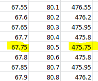
(aa) SSE() = 475.75

(bb) 100%(475.75-235)/475.75 = 50.6%

Applet Exploration: Behavior of Regression Lines

(a) Opinions may vary.

(b) Should expect this observation to “pull the line down” (smaller slope)

(c)

(d) If you pull down far enough (e.g., height < 20) then you can get the regression line to have a negative slope. This point does appear to have moderate impact on the regression line.

(e) predictions will vary

(f) The regression line does not appear to be nearly as affected by changes in the y-coordinate for this observation.

(g) (35, 60), because it has a more extreme (far from the average) x-coordinate

Excel Exploration: Minimization Criteria

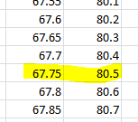
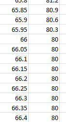
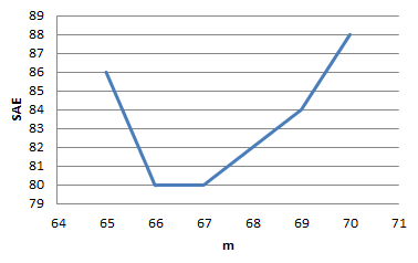
(a) SAE = 80.5

(b)

(c)

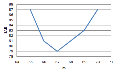
It looks like a piecewise parabola

(d) The function appears to be minimized at 67in, with an SAE value around 79.

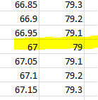
(e) There are 20 observations and 67 is the 10^th (and 11^th) value. An observation falling between the 10^th and 11^th observations is the median of the 20 values.

(f) This creates a flat spot in the graph. Now all values between 66 and 67 (inclusive) minimize the SAE at 80.

(g) This just moves the graph up (with the same shape) to higher SAE values. The optimal m is still 67 with an SAE value of 82.

(h) The median (or any value between the 10^th and 11^th sorted values)

(i) The values of the SAE would change, again proportionally, and the optimal m would remain the same.

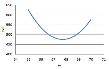
(j) This was the mean, here 67.75 in

(k) This is now a parabola, minimized at m = 67.75in (the sample mean) with an SSE value of 475.75

(l) This changes the function quite a bit and the optimal m is no longer displayed in the graph.

Investigation 4.9: Money Making Movies

(a) The observational units at the movies, the explanatory variable is the critics’ score (quantitative) and the response variable is the box office revenue (quantitative).

(b)

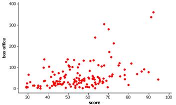
If we treat box office revenue as the response variable there is a moderate positive linear relationship between box office revenue and the critics score.

These movies had much higher box office revenues than we would have predicted based on the critics’ score.

(d) The correlation coefficient is r = 0.424 indicating a moderately strong, positive linear relationship.

(e) The regression equation is predicted box office = - 42.9 + 1.86 score

The intercept is the predicted revenue if the critics’ composite score is 0.

The slope is the predicted increase in box office revenues for a 1 point increase in the critics’ score.

(f) r² = 18% indicating that the regression on the critics score explains 18% of the variation in the box office revenues.

(g)

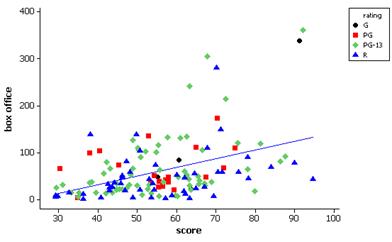
Most of the R movies are below the line. There are only a few G movies. The PG movies tend to be above or very close to the line. (Observations may vary a bit).

(h)

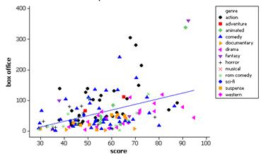
Most of the action movies appear above the line. Most of the dramas appear below the line. (Observations may vary a bit).

(i)

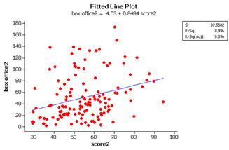
(j) The relationship now appears much weaker (r = .299, only 8.9% of variation explained) but is still positive and linear. Those 6 movies had the effect of making the overall relationship look stronger.

Investigation 4.10: Running Out of Time

(a) The explanatory variable of interest here is age and the response variable is finishing time.

(b) We might expect older people to tend to be slower (larger finish times) so a positive association. Conjectures about form and strength will vary.

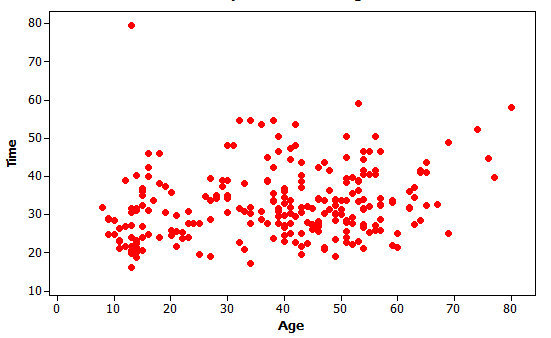
We do notice a moderate, positive, linear association between time and age. There is also an extreme outlier – a rather young runner who took almost 80 minutes. The outlier could be due to an injury during the race?

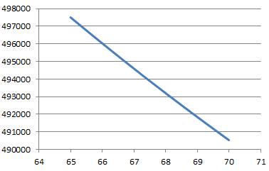
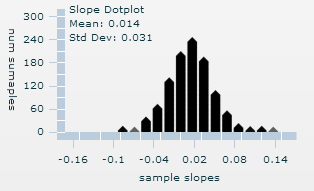
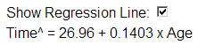
(d) Minitab fitted line plot

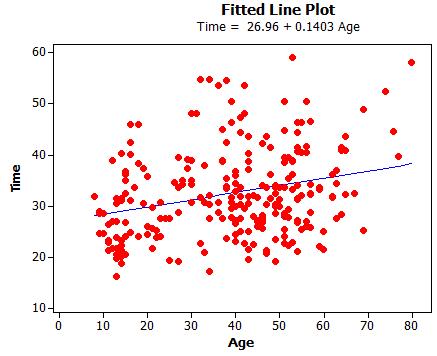
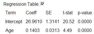
With each one-year increase in age, we predict .1403 hours (about 8 minutes) to be added to the finish time, on average.

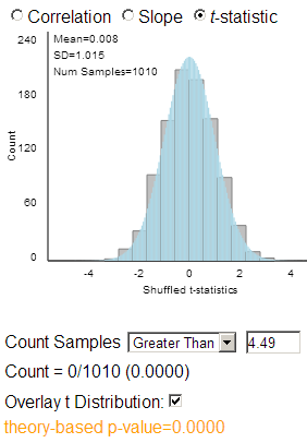
(e) It’s possible. We need to know how unusual a slope of .1403 (or more extreme) is for a sample of 247 runners from a population with no association.

(f) This would imply a population slope of zero. H₀: no association between finish time and age vs. H_a: a positive association between finish time and age (population slope > 0).

(g) Note: I removed the runner, not just the finishing time.

(h) The sample regression line shouldn’t exactly match the population regression line (b = 0)

(i) The sample regression line is expected to vary from sample to sample

(j) The lines form a criss-crossing pattern, like a bow-tie

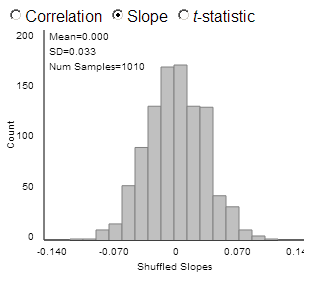
(k) The shape should be symmetric with a mean around zero and a standard deviation of about 0.03

(l) We expect the average sample slope to be close to zero, the value of the population slope. This shows that the sample slope is an unbiased estimator of the population slope.

(m) The vertical distances from the points to the horizontal regression line will be smaller.

(n) Conjectures will vary.

(o) There should be less sample-to-sample variability in the sample slopes (smaller standard deviation).

(p) The horizontal distances from the points to the value will be smaller (less horizontal width to the population scatterplot). Predictions will vary.

(q) There will actually be more sample-to-sample variability in the sample slopes (larger standard deviation).

(r) Might conjecture the sampling distribution to have less variability when the samples are based on larger sample sizes.

(s) The standard deviation of the slopes should decrease.

(t) With a larger value of , there is more variability in the distribution of sample slopes.

With a larger value of s_x, there will be less variability in the distribution of sample slopes.

With a larger sample size, there will be less variability in the distribution of sample slopes.

(u) When there is less variation away from the regression line, there will be less variation in the sample regression lines, it is more difficult to get “extreme” regression lines. When there is less variability in the explanatory variable, we are not given as much information about the relationship between the two variables and it will be easier to get more extreme sample results. Larger samples, as always, lead to less sampling variability.

(v) Yes, n and s_X² are in the denominator and s is in the numerator.

(w) Example results

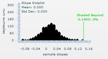
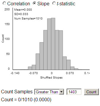
0.14 is in the tail of the simulated null distribution, it does not seem likely that if the population slope was zero we would observe a sample slope as extreme as 0.140 just by chance.

(x) Example results

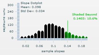
The distribution of sample means will now center around 0.10. Now the value of 0.14 is not so extreme. Here we found such a slope or larger about 10% of the time. The value of 0.10 appears to be plausible for b.

(y) Suggestions will vary.

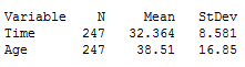
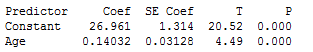
(z) By hand: t = .14/.03 » 4.67, which will have a small p-value (df = 247-2 = 245).

Minitab output:

Investigation 4.11: Running Out of Time (cont.)

(a)

(b) The slope will most likely be smaller than observed (as well the correlation coefficient, indicating a weaker association)

(c) You should get a negative association about half the time, but probably never one as extreme as the observed slope (red line)

(d) Example results

The shape is rather symmetric, centered around zero, with a standard deviation of about 0.03. This is similar to what we saw in Investigation 4.10.

(e) Example results

None of the simulated slopes was as extreme as the observed sample slope.

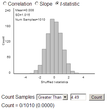
(f) If we standardize, we again get something like (0.14-0)/.03 » 4.67.

Using an observed t statistic of 4.49, we are again on the right edge of the distribution.

(g) Yes

(h)

Investigation 4.12: Boys’ Heights

(a) Explanatory variable is age and the response variable is height.

(b) We expect there to be variability in the boys’ heights within ages but we also expect a tendency for the 3 year old boys to be taller than the 2 year old boys in general.

(d) We could investigate what the lines look like when we choose random samples from a population where we know the population slope is equal to zero.

(e)

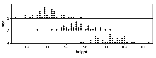
The distributions look roughly normal with similar variability but different centers. The means each differ by about 6.

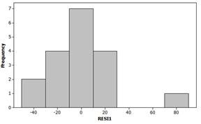
(f) These conditions do appear to be met for the Berkeley boys’ heights. We have a normal distribution at each x and the spread of each distribution is similar.

Investigation 4.13: Cat Jumping (cont.)

(a) Minitab results for predicted velocity

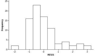
(b) Minitab output

It’s hard to tell much with a small sample size and we do have the one extreme outlier, but otherwise, the normality condition would appear satisfied.

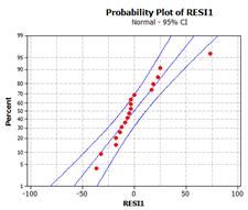
(c)

If we separate the one huge outlier, the remaining residuals are in a rectangular box from -25 to 25. The lack of any strong curvature indicates the linearity condition is reasonable and the lack of major “fanning” in the residuals indicates the equal variance condition is met.

(d) Let b represent the population slope between takeoff velocity and percentage body fat for all cats.

H₀: b = 0 (no association between takeoff velocity and percentage body fat in the population)

H_a: b < 0 (negative association)

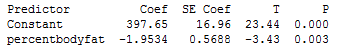
With a t-statistic of -3.343 and a p-value of 0.003 < .05, we would reject the null hypothesis at the 5% level of significance and conclude that we have convincing evidence of a negative association between percentage body and takeoff velocity in this population of cats.

(e) t = -1.9534/.5688 » -3.43.

(f) If we use 2 as the critical value, we would find -1.9534 + 2(.5688) which gives (-3.091, -0.8158)

If we use a t critical value for 95% confidence and 18-2 = 16 d.f, we would find -1.9534 + 2.1199(.5688) which gives (-3.1592, -0.7476)

(g) We are 95% confident that each one percentage point increase in body fat is associated with a .75 to 3.16 decrease in takeoff velocity (cm/sec).

(h) 25%: predicted velocity = 397.65 – 1.9534 (25) » 248.82 cm/sec.

50%: 299.98 cm/sec

(i) Should have more faith in the prediction for 25% body fat as that value is in the main part of our data but we don’t have a lot of information for cats with body fat percentages around 50%.

(j) Minitab output:

Midpoint is our prediction of 248.82. We are 95% confident that the takeoff velocity for a cat with 25% body fat will be between 292.37 cm/sec and 205.26 cm/sec.

(k) Minitab output:

The midpoint is lower (now at 299.98) but the width is 362.34-237.62 = 124.72 (compared to 405.26-292.37 = 112.89) is larger. This makes sense because we don’t expect predictions at 50% body fat to be as precise.

(l) Minitab output

The midpoint is the same (248.82). We are 95% confident that the average takeoff velocity for all cats with 25% body fat is between 335.45 and 262.19 cm/sec.

(m) The interval is narrower because it is easier to predict an average than an individual observation.

Investigation 4.14: Housing Prices

(a) The regression equation is predicted price = 65930 + 202 square foot. r² = 42.1%

(b) Yes

(c)

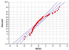
The residuals appear to be skewed to the right and not following a normal distribution.

(d)

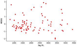
There does not appear to be strong curvature but the spread does appear to increase across the graph.

(e)

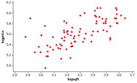
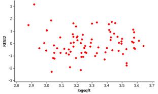
Although not perfect, these variables do appear to better follow the basic regression model. The residuals appear less skewed and there is less variation in the “width” of the residuals at different values of the explanatory variable. There does not appear to be any curvature in the relationship either.

(f) The regression equation is predicted logprice = 2.70 + 0.890 logsqft. If the log square footage increases by one (which corresponds to a ten-fold increase in square footage), we predicted the log price will increase by .890 (which corresponds to a 10^.89-fold increase in price). If the log square footage is equal to 0 (square footage = 1), the predicted log price is 2.70 (price = 10^2.70).

(g) predicted logprice = 2.70 + .890 logten(3000) = 5.79

So the predicted price is 10^5.79 = $623,215.

Technology Exploration: The Regression Effect

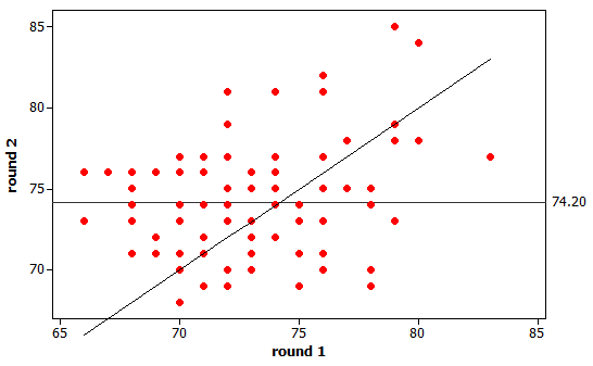
(a) r = 0.246

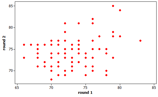
There is a weak, linear, positive association between the round1 and round2 scores.

(b) Top ten:

Marc Leishman	66	73
Sergio Garcia	66	76
Dustin Johnson	67	76
Matt Kuchar	68	75
Fred Couples	68	71
Gonzalo Fernandez-Castano	68	74
Rickie Fowler	68	76
David Lynn	68	73
Trevor Immelman	68	75
Adam Scott	69	72

Bottom ten:

Branden Grace	78	70
Michael Weaver	78	74
Padraig Harrington	78	75
Thaworn Wiratchant	79	73
Tom Watson	79	78
Craig Stadler	79	79
Hiroyuki Fujita	79	85
Ian Woosnam	80	78
Ben Crenshaw	80	84
Alan Dunbar	83	77

For the bottom ten: One golfer tied his first round score and two did worse, everyone else improved

(d) The bottom ten group saw substantially more (7 vs 0) people improve.

(e) The median (sorting first) round 2 score for the top ten is 74.5 and for the bottom ten it’s 77.5. The top ten golfers tended to score better in the second round.

(f) Tiger Woods

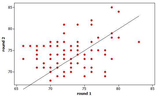
(g) The line doesn’t really go through the “middle” of the points. It’s too low for small round 1 scores and too high for larger round 1 scores.

Expect the regression line to have a smaller slope.

(h)

This line does not summarize the relationship well. It’s a little too high for lower round 1 scores and too low for higher round 1 scores. We expect the regression line to have a larger slope.

(i) The regression line falls “in between” the other two lines

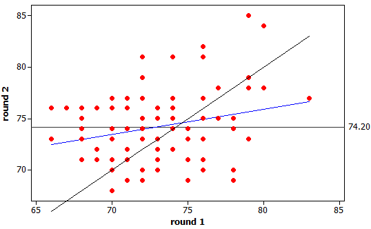
(j) The regression slope of .2428 is less than one, in fact very close to the value of r.

(k) We expect poor first round scores to be below the mean but not by as much. We expect good (low) first round scores to be followed by second round scores that are above the mean but not by as much (by a fraction).