


Despite this lack of thoroughness, we hope that this guide will prove useful to instructors. For a more complete perspective, you should use these answers in conjunction with the Guide for Instructors, which offers suggestions on what to look for and to emphasize in each in-class activity.
This page contains a large number of graphics, but you can also access a Text-Only Version.
This document is fairly lengthy, and this should be kept in mind if a print out is to be made.


(a)
gender: categorical (binary)
politcal identification: categorical
penny question: categorical (binary)
value of statistics: measurement
number of states: measurement
number of countries: measurement
Europe?: categorical (binary)
WDW?: categorical (binary)
letters per word: measurement
(b) categorical
(c) measurement
(a) - (d) These answers depend on class results.
| Rating | 1 | 2 | 3 | 4 | 5 | 6 | 7 | 8 | 9 |
|---|---|---|---|---|---|---|---|---|---|
| Tally (count) | These answers depend on class results. | ||||||||
(a) - (d) These answers depend on class results.
(a)
| Specialty | Percentage Women | Specialty | Percentage Women | |
|---|---|---|---|---|
| Aerospace medicine | 5.93% | Nuclear medicine | 15.74% | |
| Allergy & immunology | 16.04% | Obstetrics/gynecology | 25.61% | |
| Anesthesiology | 18.37% | Occupational medicine | 11.55% | |
| Cardiovascular disease | 5.55% | Opthamology | 10.60% | |
| Child psychiatry | 35.45% | Orthopedic surgery | 2.49% | |
| Colon/rectal surgery | 3.34% | Otolaryngology | 5.86% | |
| Dermatology | 24.09% | Pathology-anat./clin. | 24.44% | |
| Diagnostic radiology | 16.80% | Pediatric cardiology | 20.29% | |
| Emergency medicine | 15.25% | Pediatrics | 41.01% | |
| Family practice | 19.05% | Physical med./rehab. | 30.10% | |
| Forensic pathology | 23.17% | Plastic surgery | 7.12% | |
| Gastroenterology | 6.39% | Psychiatry | 24.80% | |
| General practice | 11.24% | Public health | 24.14% | |
| General preventive medicine | 25.43% | Pulmonary diseases | 8.84% | |
| General surgery | 7.22% | Radiation oncology | 18.79% | |
| Internal medicine | 21.79% | Radiology | 9.99% | |
| Neurological surgery | 3.24% | Thoracic surgery | 1.42% | |
| Neurology | 16.75% | Urological surgery | 1.71% |
(b)
Three highest: pediatrics, child psychiatry. and physical med./rehab.
Three lowest: thoracic surgery, urological surgery, and orthopedic
surgery
(c)

(d) (Asks for interpretation)

(a) The centers of these distributions vary.
(b) The spreads of these distributions vary.
(c) The shapes of these distributions vary.
(d) This distribution has two distinctive clusters.
(e) This distribution has two outliers- one very low score and one very
high.
(f) This distribution reveals granularity in that scores occur only in multiples of five.
(a) 63;
Victoria
(b) 0;
Edward V;
he ruled for some short period less than a year
(c)
0 | 9 0 2 6 5 3 6 7 9 1
1 | 3 9 0 7 3 3 2 3 0 5
2 | 1 0 2 2 4 2 4 5 5
3 | 5 5 5 9 8 3
4 | 4
5 | 6 0 9
6 | 3
(d)
0 | 0 1 2 3 5 6 6 7 9 9
1 | 0 0 2 3 3 3 3 5 7 9
2 | 0 1 2 2 2 4 4 5 5
3 | 3 5 5 5 8 9
4 | 4
5 | 0 6 9
6 | 3
(e) f
(f) 19.5
(g) 9.5
(h) 34
2-3: Pennsylvania College Tuitions
(a) 16
(b) 16; .1019
(c)
skewed to the right
(d) There are roughly three clusters or peaks, perhaps corresponding to public institutions and two classes of private ones.
These answers depend on class results.

(a)

(b)
Many reasonable answers are acceptable.
(c)
76/9 (approx. 8.44)
(d)
more: 3;
less: 6
(e)
6
(f) more: 4;
less: 4
(g) the fifth
(h) n=5: the third
n=7: the fourth
n=9: the fifth
n=11: the sixth
n=13: the seventh
(i) the ((n+1)/2)th
(a) 1 3 6 6 7 15 28 31
(b) 12.125
(c) 6
(d) There are an even number of observations, so none falls right in the middle.
(e) 6.5
(a) (Asks for prediction)
(b)
| Class A | Class B | Class C | |
|---|---|---|---|
| Mean | 80.55 | 69.38 | 60.26 |
| Median | 81 | 70 | 61 |
(c) - (e) (Asks for prediction)
(f)
| Class G | Class H | Class I | |
|---|---|---|---|
| Mean | 49.77 | 50.61 | 51.20 |
| Median | 49 | 49 | 53 |
(g)
The mean and median are close together for symmetric distributions. The
mean exceeds the median for distributions skewed to the right, and the
mean is less than the median for distributions skewed to the left.
(h) - (i) see table below
(j)
| Mean | Median | |
|---|---|---|
| Justices | 8.44 | 6 |
| Justices with "big outlier | 10.67 | 6 |
| Justices with "huge" outlier | 30.67 | 6 |
(k)
The median is resistant.
(l) no
(m) No, it does not make sense to talk about the mean or median gender. The mode of the genders is sensible, for it is the more frequent gender.
3-4: Readability of Cancer Pamphlets
(a)
We do not know the actual reading levels of the 6 patients in the "under
3"
category and the 17 patients in the "above 12" category..
(b) 9
(c) 9
(d) The medians are the same.
(e) no
(f) 17/63
3-5: Students' Distances from Home
(a) - (e)
These answers depend on class results.
(f)
no

(a)

(b)
mean = 8.44;
median = 6
(c)
22
(d) 0 1 3 4; lower quartile = 2
(e) 8 13 19 22; upper quartile = 16
(f)
IQR = 14
(g)
| Original Data | Deviation from mean | Squared deviation | |
|---|---|---|---|
| 22 | 13.56 | 188.75 | |
| 19 | 10.56 | 111.42 | |
| 13 | 4.56 | 20.79 | |
| 8 | -0.44 | 0.20 | |
| 6 | -2.44 | 5.95 | |
| 4 | -4.44 | 19.75 | |
| 3 | -5.44 | 29.64 | |
| 1 | -7.44 | 55.42 | |
| 0 | -8.44 | 71.31 | |
| Column sum | 76 | .04 | 503.23 |
(h)
7.89
(i)

4-2: Properties of Measures of Spread
(a) (Asks for prediction)
(b)
| Class D | Class E | Class F | |
|---|---|---|---|
| Std. dev. | 2.837 | 7.018 | 11.78 |
| IQR | 3 | 9 | 13.75 |
(c) - (d) see table below
(e)
| Std. dev. | IQR | |
|---|---|---|
| Justices | 7.89 | 14 |
| Justices with "big" oultier | 13.21 | 14 |
| Justices with "huge" outlier | 72.0 | 14 |
(f) The interquartile range is resistant. The standard deviation and range are not resistant.
(a) yes
(b) (6.362, 14.080)
(c)
146; 0.685
(d)
202; 0.948
(e) 213; 1.000
(a) 184
(b) 7.4
(c)
no
(d)
1.057
(e)
1.423
(f)
Kathy
(g) (Asks for interpretation)
(h)
Mike: -0.897; Karen: -0.308
(i) Karen
(j)
The z-score turns out to be negative when the raw score is less than the
mean score.

(a)
| State | % change | Region | State | % change | Region | |
|---|---|---|---|---|---|---|
| Alabama | 3.6 | E | Montana | 5.1 | W | |
| Alaska | 8.9 | W | Nebraska | 1.8 | W | |
| Arizona | 7.4 | W | Nevada | 15.6 | W | |
| Arkansas | 3.1 | W | New Hampshire | 1.4 | E | |
| California | 3.7 | W | New Jersey | 1.9 | E | |
| Colorado | 8.2 | W | New Mexico | 6.7 | W | |
| Connecticut | -0.3 | E | New York | 1.1 | E | |
| Delaware | 5.1 | E | North Carolina | 4.8 | E | |
| Florida | 5.7 | E | North Dakota | -0.6 | W | |
| Georgia | 6.8 | E | Ohio | 2.3 | E | |
| Hawaii | 5.7 | W | Oklahoma | 2.7 | W | |
| Idaho | 9.2 | W | Oregon | 6.7 | W | |
| Illinois | 2.3 | E | Pennsylvania | 1.4 | E | |
| Indiana | 3.0 | E | Rhode Island | -0.3 | E | |
| Iowa | 9.2 | W | South Carolina | 4.5 | E | |
| Kansas | 2.1 | W | South Dakota | 2.8 | W | |
| Kentucky | 2.8 | E | Tennessee | 4.5 | E | |
| Louisiana | 1.9 | W | Texas | 6.2 | W | |
| Maine | 0.9 | E | Utah | 7.9 | W | |
| Maryland | 3.8 | E | Vermont | 2.3 | E | |
| Massachusetts | -0.1 | E | Virginia | 4.9 | E | |
| Michigan | 2.0 | E | Washington | 8.0 | W | |
| Minnesota | 3.3 | W | West Virginia | 1.5 | E | |
| Mississippi | 2.7 | E | Wisconsin | 3.0 | E | |
| Missouri | 2.3 | W | Wyoming | 3.7 | W |
(b) 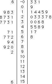
(c)
East: 2.5;
West: 4.4
(d)
This answer varies from student to student.
(e) The West tends to have a higher percentage change.
(f) No; there are many possible pairings.
(g) The West.
5-2: Professional Golfers' Winnings
(a)
| Tour | Minimum | Lower quartile | Median | Upper quartile | Maximum |
|---|---|---|---|---|---|
| PGA | 435 | 809 | 658 | 495 | 1165 |
| LPGA | 122 | 301 | 186 | 149 | 863 |
| Senior | 208 | 568 | 340 | 265 | 1190 |
(b)
 |
 |
 |
(c) no
(d)
PGA: no outliers
LPGA: three outliers: 863, 732, 543
(e)
 |
 |
 |
(f)
yes
(g) (Asks for interpretation)
(a) - (d) These answers depend on the class
results.

(a)
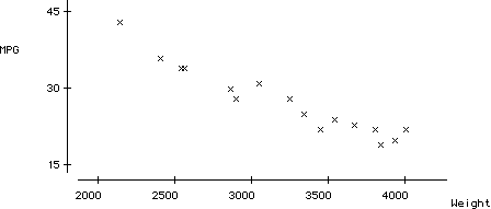
(b) Heavier cars tended to get worse fuel efficiency.
(c) negatively
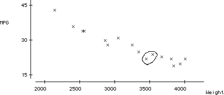
(d) yes; there are many such pairs.
(a)
Students who did well on the first test tended to do well on the second,
and those
who did poorly on the first tended to do poorly on the second.
(b)
| Most strong | Moderate | Least strong | |
|---|---|---|---|
| Negative | C | D | F |
| Positive | E | A | B |
(c) (Asks for interpretation)
(a) yes; positive; fairly strong
(b)
2
(c) 16
(d)
6
(e) One can discover that for most of these couples, the husband is older than the wife.
(a)
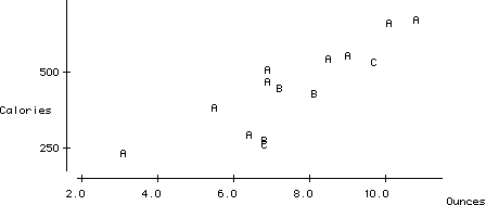
A- roast beef
B - chicken
C - turkey
(b)
There is a reasonably strong, positive association between a sandwich's
serving
size and its calories.
(c) Roast beef sandwiches tend to have more calories per serving size than do chicken and turkey sandwiches.
6-5: Space Shuttle O-Ring Failures
(a)
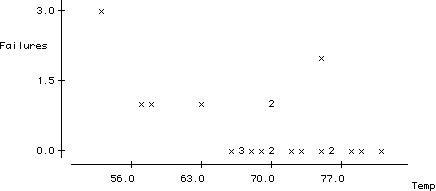
The scatterplot reveals a weak-to-moderate negative association between
temperature and O-ring failures.
(b)
The likelihood of O-ring failure appears to be greater at such a low
temperature.
(c)
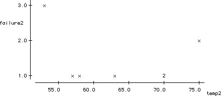
The association is much weaker in this case.
(d)
(Asks for interpretation)
<

(a)
| Strong | Moderate | Least Strong | |||||||
|---|---|---|---|---|---|---|---|---|---|
| Negative |
|
|
| ||||||
| Positive |
|
|
|
(b)
largest: 1;
smallest: -1
(c) The data would have to fall exactly on a straight line.
(d)
The sign of the correlation (positive or negative) matches the direction
of
the association.
(e)
The stronger the association, the closer the correlation comes to �1.
The weaker the association, the closer the association comes to 0.
(f) The data reveal a distinct curvilinear relationship.
(g)
0
(h)
Yes, except for the person who scored very high on the first exam and
very low on the second.
(i)
Yes, except for the person who scored very low on both exams.
(j)
H: 0.037;
I: 0.705
(k)
H: 1.000;
I: 0.130;
These correlations have changed substantially.
(l)
No, because it can be strongly affected by outliers.
(m)
There are two distinct clusters, one with students doing poorly on
both exams and another with students doing well on both exams.
(n)
.954
7-2: Televisions and Life Expectancy
(a) fewest: United States, 1.3;
most: Haiti, 234
(b)
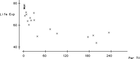
(c)
-.804
(d) (Asks for interpretation)
(e) no
(f) (Asks for interpretation)
7-3: Cars' Fuel Efficiency ( cont. )
(a)
| Model | Weight | Weight z-score | MPG | MPG z-score | Product |
|---|---|---|---|---|---|
| BMW 3-Series | 3250 | 0.07 | 28 | 0.07 | 0.00 |
| BMW 5-Series | 3675 | 0.79 | 23 | -0.68 | -0.54 |
| Cadillac Eldorado | 3840 | 1.07 | 19 | -1.28 | -1.37 |
| Cadillac Seville | 3935 | 1.23 | 20 | -1.13 | -1.39 |
| Ford Aspire | 2140 | -1.81 | 43 | 2.30 | -4.17 |
| Ford Crown Victoria | 4010 | 1.36 | 22 | -0.83 | -1.13 |
| Ford Escort | 2565 | -1.09 | 34 | 0.96 | -1.05 |
| Ford Mustang | 3450 | 0.41 | 22 | -0.83 | -0.34 |
| Ford Probe | 2900 | -0.52 | 28 | 0.07 | -0.03 |
| Ford Taurus | 3345 | 0.23 | 25 | -0.38 | -0.09 |
| Ford Taurus SHO | 3545 | 0.57 | 24 | -0.53 | -0.30 |
| Honda Accord | 3050 | -0.27 | 31 | 0.51 | -0.14 |
| Honda Civic | 2540 | -1.13 | 34 | 0.96 | -1.09 |
| Honda Civic del Sol | 2410 | -1.35 | 36 | 1.26 | -1.70 |
| Honda Prelude | 2865 | -0.58 | 30 | 0.36 | -0.21 |
| Lincoln Mark VIII | 3810 | 1.02 | 22 | -0.83 | -0.83 |
(b) -.96
(c)
The cars with negative wieght z-scores tend to have positive MPG z-scores,
and vice versa.
(a) - (c)
The answers vary from student to student.

(a) - (e) The answers vary from student to student.
(a)
| Mean | Std. dev. | Correlation | |
|---|---|---|---|
| Airfare (y) | 166.9 | 59.5 |
|
| Distance (x) | 713 | 413 |
(b)
b = 0.117;
a = 83.3
(c) airfare = 83.3 + .117 distance
(d) 118.50
(e)
259.30
(f)
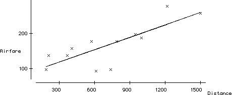
(g)
(Asks for prediction)
(h)
188.90
(i)
416.80
(j)
| Distance | 900 | 901 | 902 | 903 |
|---|---|---|---|---|
| Predicted Airfare | 188.90 | 189.02 | 189.13 | 189.25 |
(k) yes; 0.117; this number is the slope coefficient of the least squares line.
(l) 11.70
(m)
150.88
(n) 27.12
(o)
| Destination | Distance | Airfare | Fitted | Residual |
|---|---|---|---|---|
| Atlanta | 576 | 178 | 150.88 | 27.12 |
| Boston | 370 | 138 | 126.70 | 11.30 |
| Chicago | 612 | 94 | 155.10 | -61.10 |
| Dallas/Fort Worth | 1216 | 278 | 226.00 | 52.00 |
| Detroit | 409 | 158 | 131.27 | 26.73 |
| Denver | 1502 | 258 | 259.57 | -1.56 |
| Miami | 946 | 198 | 194.30 | 3.70 |
| New Orleans | 998 | 188 | 200.41 | -12.41 |
| New York | 189 | 98 | 105.45 | -7.45 |
| Orlando | 787 | 179 | 175.64 | 3.36 |
| Pittsburgh | 210 | 138 | 107.92 | 30.08 |
| St. Louis | 737 | 98 | 169.77 | -71.77 |
(p)
St. Louis;
distance: 737
airfare: 98;
residual: 71.77;
overestimate
(q)
greater
(r)
below
(s)
mean: 0;
standard deviation: 36.1
(t)
0.368
(u)
0.632
(v)
The sum equals one.
(w)
.632
8-3: Students' Measurements ( cont. )
(a) - (e) These answers depend on class results.
(f)
no

(a)
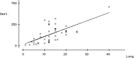
Gestation = 21.7 + 13.1 Longevity
(b)
For every additional year of longevity, one expects the animal's gestation
period to increase by 13.1 days.
(c)
.44
(d)
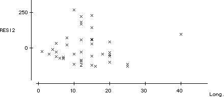
(e)
elephant;
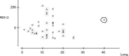
No, the elephant does not have the largest residual.
(f)
giraffe;
longer
(g)
Gestation = 9.0 + 13.6 Longevity; 50.1%
(h) no
(i)
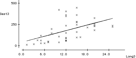
Gestation = 45.0 + 11.1 Longevity; 26.9%
(j) The removal of the elephant affected the graph more.
(k)
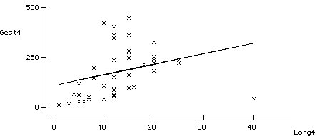
Gestation = 110 + 5.26Longevity
r^2 = .092
9-2: Planetary Measurements ( cont. )
(a) (Asks for interpretation)
(b)
0.910, a very strong, positive correlation which seems to indicate a
strong linear relationship.
(c)
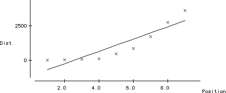
Distance = -1126 + 446 Position
(d)
No, the line does not fit that data well. The line does not
capture the curved aspect of the relationship.
(e)
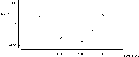
Yes, the residual plot reveals a clear, curved pattern.
9-3: Televisions and Life Expectancy ( cont. )
(a)
 <
<
r = -0.804; the relationship does not appear to be linear
(b)

(c)
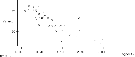
r = -0.855; the relationship appears to be stronger and more linear.
(d)
life expectancy = 77.9 - 9.81Log(PerTV)
(e)
85.1%
(f)
55
(g)
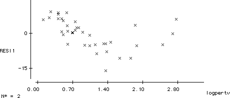
no
(h)
The transformed data produces a better fit than the original data.

(a)
| Category pair | Tally |
|---|---|
| Retain, liberal |
|
| Retain, moderate | |
| Retain, conservative | |
| Abolish, liberal | |
| Abolish, moderate | |
| Abolish, conservative |
(b)
| Retain | Abolish | |
|---|---|---|
| Liberal | | |
| Moderate | ||
| Conservative | ||
10-2: Age and Political Ideology
(a)
0.205
(b)
0.388
(c)
0.406
(d)
0.280
(e)
0.473
(f)
0.247
(g)
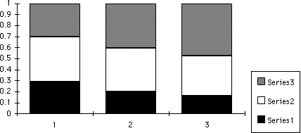
Series 1 - Liberal
Series 2 - Moderate
Series 3 - Conservative
(h) (Asks for interpretation)
(i)
0.473
(j)
0.199
(k)
0.097
(a) (Asks for prediction)
(b)
AZT: 0.079;
HIV: 0.250
(c)
3.23
(d) (Asks for interpretation)
10-4: Hypothetical Hospital Recovery Rates
(a)
A: 0.8;
B: 0.7; B saves the higher percentage.
(b)
Are you convinced?
(c) A: 0.983;
B: 0.967; A saves the higher percentage.
(d)
A: 0.525;
B: 0.3; A saves the higher percentage.
(e)
Hospital A tends to treat the large majority of patients in "poor"
condition.
Since these patients are more likely to die than those in "good"
condition,
A's overall survival rate is lower than B's despite being higher for each
type of patient.
(f) Hospital A is preferable regardless of one's condition.
10-5: Hypothetical Employee Retention Predictions
(a)
0.16
(b)
0.16
(c)
no
(d)
no
(e)
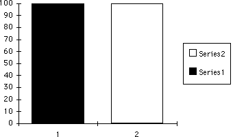
Series 1 - Predicted to stay
Series 2 - Predicted to leave
(f)
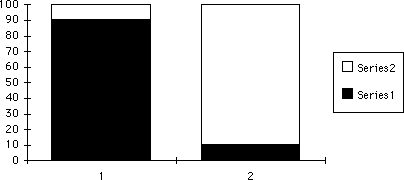
Series 1 - Predicted to stay
Series 2 - Predicted to leave

(a)
No; those with more passionate views of Elvis are more likely to pay to
voice their opinions.
(b) One flaw is that those with telephones or vehicles in 1936 tended to be the more affluent segment of society. Another flaw is that those who took the time to respond probably tended to be less satisfied with the incumbent.
(c)
Elvis: population - all American adults, sample - those radio listeners
who chose to pay to call in
station
Literary Digest: population - all American adults, sample - those who
received the questionnaire and chose to respond
(a)
Gender: categorical (binary)
Party: categorical (binary)
State: categorical
Years of service: measurement
(b) - (e)
These answers vary from student to student.
(f) no; no; almost certainly no
(g)
No, the random sampling method is not biased because it does not
systematically under- or over-represent certain groups.
(h) You would have to use three-digit labels for the representatives, read
off three digits at a time from the table, and ignore numbers from 436 to
999 and 000.
(i)
 = .93
= .93


 = 8.72
11-3: Sampling U.S. Senators ( cont. )
(a) - (f)
Answers vary.
(g) sample size of 10
(h)
sample size of 40
(i)
the population mean of 12.54
(j)
no

(a) Answers vary.
(b)
statistic, 
(c)
parameter, 
(d)
no
(e)
yes, answers vary.
(f)
no;
sampling variability
(g)
Answers vary.
(h) no (almost surely)
(i) no (almost surely)
(j)
Answers vary.
(k)
yes;
yes;
(l)
more spread out
(m) less spread out
12-2: Simulating Reese's Pieces
(a)
Answers vary.
(b)
Distribution of sample proportion should be roughly mound shaped,
symmetric, and centered in the neighborhood of 0.45.
(c)
Answers vary.
(d)
yes
(e) Answers vary.
(f)
This should be the middle percentage from the table.
(g) no; yes; Since most (about 95%) sample proportions fall within .20 of the population proportion, it is quite likely that a particular sample proportion will fall within .20 of the population proportion.
(h)
Answers vary.
(i) less spread out but roughly same shape and center
(j)
Answers vary.
(k)
There should be a higher percentage of sample proportions falling
within �.10 of .45 with samples of 75.
(l)
larger sample size
(m) - (n) Answers vary.
(o)
95%
(p) Mean: .45; Standard deviation: .0995
(q) Mean: .45;
Standard deviation: .0574

(a)
parameter;

(b)
 =4/15
=4/15
(c) yes
(d) no; sampling variability
(e) - (g) Answers vary.
(h)
no (almost surely)
(i) - (j)
Answers vary.
(k)
no
(l) - (m) Answers vary.
(n)
no
(o) no
13-2: Widget Manufacturing ( cont. )
(a)
Answers vary.
(b) yes
(c) Answers vary. The evidence of improvement is even stronger here.
(a) 0
(b) 4797; 47.97%
(c)
According to the simulation, the chance of getting nine or more correct by
guessing is around 32.09%, not very surprising.
(d)
According to the simulation, the chances of getting twelve or more correct
is around 5.05%, moderately surprising.
(e)
According to the simulation, the chances of getting fifteen or more
correct is around .24%, very surprising.
(f)
Only about 3 of every 10,000 subjects would get seventeen or more
correct by guessing. This constitutes strong evidence that the
person actually possesses some special ability.

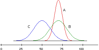
(a) roughly symmetric, mound shaped
(b)

(c)
14-2: Standard Normal Calculations
(a)
.7517
(b)
.7517
(c)
.2483
(d)
.0838
(e)
.6679
(f)
less than .0002
(g)
k = 1.28
(h)
k = 1.53
(a) (Asks for prediction)
(b)
-1.00
(c)
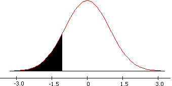
(d) .1587
(e) .9332
(f)
.5007
(g)
0.1%
(h) 139.96

(a)
normal distribution with mean .45 and standard deviation .0574
(b)
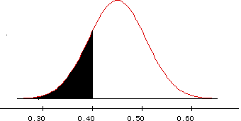
(c) .1922
(d) .9182
(e)
They should be close.
(a)
normal distribution with mean .25 and standard deviation .0791
(b)
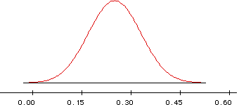
(c)
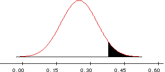
(d) .0505
(e) 12 or more correct: 505/10000. They are amazingly close.
(f) Reasonably but not terribly surprising; yes; no
(a)
normal distribution with mean .45 and standard deviation .0376;
same shape and center but less spread out
(b) 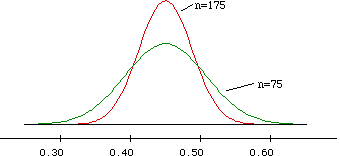
(c) 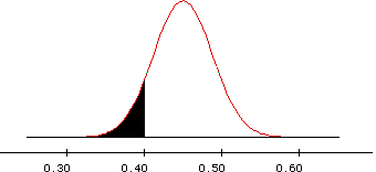
(d) .0918; smaller probability
(e)
.9922; larger probability

(a)
Answers vary.
(b)
statistic;

(c) no
(d) yes
(a)
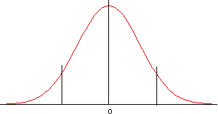
(b) .975
(c) 1.96
(d) z* = 1.44
16-3: Penny Spinning ( cont. )
(a)
Answers vary.
(b)
no
(c) - (d) Answers vary.
(e)
look at 
(f) Simple random sampling, large sample size
(a) - (c)
Answers vary.
(d)
no
(e) 95% of all intervals geberated by this procedure do contain the actual parameter value.
16-5: Effect of Confidence Level
(a) (Asks for prediction)
(b) Answers vary , but the intervals
should get gradually wider (with the same center).
(c) Requiring less confidence allows for a narrower interval.
(a) (Asks for prediction)
(b)
| Sample Size | Sample heads | Confidence interval | Half-width | Width |
|---|---|---|---|---|
| 100 | 35 | (.257, .443) | .093 | .156 |
| 400 | 140 | (.303, .397) | .047 | .094 |
| 800 | 280 | (.317, .383) | .073 | .066 |
| 1600 | 560 | (.327, .373) | .023 | .046 |
(c)
The intervals get narrower as the sample size gets larger.
(d) twice as big
(e)
cuts the half-width in half

(a) (.7294, .7906)
(b) simple random sample; large sample size
(c) .0306
(d)
This margin of error comes from the half-width of the 95% confidence
interval.
(e)
(f) (Asks for prediction)
(g) .0187; .0419
(h) The margin-of-error decreases as the sample size increases.
(i)
Greater, since the sample size of men only would be smaller than that
of the complete sample.
(j) Greater, since the sample size of male college graduates would be smaller than that of the complete sample.
17-2: Congressional Term Limits
(a) need 601 people (rounded up from 600.25)
(b) (Asks for prediction)
(c) 9604
(d) (Asks for prediction)
(e) 16,590
(f) not at all
(g)
| Case | Sample size | Confidence level | C.I. half-width |
|---|---|---|---|
| 1 | Fixed | Increases | Increases |
| 2 | Fixed | Increases | Increases |
| 3 | Increases | Fixed | Decreases |
| 4 | Decreases | Fixed | Increases |
| 5 | Increases | Increases | Fixed |
| 6 | Increases | Increases | Fixed |
(h) the whole population of American adults
17-3: Female Senators ( cont. )
(a)
(.02, .12)
(b) no
(c)
horribly biased sampling method
(d) No, because we know the whole population of the 1994 U.S. Senate.
17-4: College Students' Credit
(a) - (b)
Answers vary.
(c)
It is doubtful that the results would generalize to a larger population.

(a) .25
(b) no
(c) yes
(d) yes
(e) Wilma
(f) normal distribution with mean .25 and standard deviation .0433
(g) no
(h) yes
(i)
| Subject | Sample number of correct IDs | Sample proportion of correct IDs | Approx.probability of doing so well by just guessing | Your belief
that  > .25 (better than guessing) > .25 (better than guessing) |
|---|---|---|---|---|
| Fred | 28 | .28 | .2442 | none |
| Barney | 31 | .31 | .0829 | some |
| Betty | 34 | .34 | .0188 | much |
| Wilma | 37 | .37 | .0028 | very much |
(a)
 :
:  = .25
= .25
(The subject is just guessing and would get 25% right in long run.)
(b)
 :
:  > .25
> .25
(The subject does better then guessing and would get
more than 25% right in long run.)
(c) z = 1.39
(d) p-value = .0823
(e) If Barney were just guessing, he'd do this well or better about 8.23% of the time in the long run.
(f)
There is some, but not much, evidence to support the claim that Barney
does
better than just guessing.
(g)
yes; yes; no
(h)
no; no; no
(i)
| Subject | Sample proportion | Test statistic | p-value | Signif. at .10 level? | Signif. at 0.5? | Signif. at .01? |
|---|---|---|---|---|---|---|
| Fred | 0.28 | 0.69 | 0.2442 | no | no | no |
| Barney | 0.31 | 1.39 | 0.0829 | yes | no | no |
| Betty | 0.34 | 2.08 | 0.0188 | yes | yes | no |
| Wilma | 0.37 | 2.77 | 0.0028 | yes | yes | yes |
(a) parameter, since it pertains to the entire popultation of adult Americans.
(b)
 :
:  = .5;
= .5;
 :
:  > .5
> .5
(c)
statistic
(d) sample size
(e) (Asks for prediction)
(f)
| Sample size | (One-sided) p-value | Signif. at .10 level? | Signif. at .05? | Signif at .01 level? | Signif at .001 level? |
|---|---|---|---|---|---|
| 100 | .2119 | no | no | no | no |
| 300 | .0829 | yes | no | no | no |
| 500 | .0368 | yes | yes | no | no |
| 1000 | .0059 | yes | yes | yes | no |
| 2000 | .0002 | yes | yes | yes | yes |

(a)
 , the proportion of all penny spins that
would land
heads
(b)
two-sided;
you are looking at "euqally likely" without regard to more or less.
(c)
 :
:  = 0.5;
 :
:  � 0.5
� 0.5
(d) z = -1.633; p-value = .1025
(e) z = 1.633; p-value = .1025
(f) no
(g)
 :
:  = 0.5;
 :
:  < 0.5
< 0.5
(h) z = -1.633; p-value = .0512
(i) z = 1.633; p-value = .9488
(j)
The sample result is not even in the direction of the alternative
hypothesis.
(k)
| Sample Result | Alternative hypothesis | Test statistic | p-value |
|---|---|---|---|
| 65 heads, 85 tails |  � .5 � .5 | 1.633 | .1024 |
| 85 heads, 65 tails |  � .5 � .5 | -1.633 | .1024 |
| 65 heads, 85 tails |  < .5 < .5 | 1.633 | .0512 |
| 85 heads, 65 tails |  < .5 < .5 | -1.633 | .9488 |
19-2: American Moral Decline ( cont. )
(a)
(.729, .790)
(b) no
(c) - (g)
Hypothesized value of 
| Contained in 95% c.i.? | Test statistic | (Two- sided) p-value | Significant at .05 level? |
|---|---|---|---|---|
| .50 | no | 14.187 | �0 | yes |
| .70 | no | 3.543 | .0004 | yes |
| .75 | yes | 0.591 | .5575 | no |
| .78 | yes | -1.363 | .1729 | no |
| .80 | yes | -2.779 | .0055 | yes |
(h) Whenever the confidence interval includes the value, the test is not significant. Whenever the confidence interval does not include the value, the test is significant.
(a)
z = 1.556;
p-value = .0598
(b)
z = 1.697;
p-value = .0448
(c)
z = 3.394 ;
p-value = .0003
(d) a and b
(e) b and c
19-4: Tax Return Errors ( cont. )
(a)
 = .30626
(b) (Asks for prediction)
(c)
 :
:  =.3 ;
=.3 ;
 :
:  �.3
�.3
z = 3.055; p-value = .0023
(d)
(.301, .312)
(e)
no
(f)
no
(a)
z = 216.887
p-value = 0 (virtually)
(b)
(.569, 571)
(c)
The sampling procedure was horribly biased in favor of Landon.

(a) The primary difficulty is the lack of a comparison group. Several reasonable explanations can be provided.
(b)
explanatory: whether the student had coaching or not;
response: the student's improvement in SAT scores
(c) observational study
(a)
explanatory: whether the patient owns a pet or not;
response: whether the patient survives or not
(b) observational study
20-3: Vitamin C and Cold Resistance
(a)
expl: whether the subject takes vitamin C or not;
response: whether the subject resists a cold or not
(b)
controlled experiment
(c) Many reasonable answers are possible.
20-4: Pregnancy, AZT, and HIV ( cont. )
(a)
expl: whether the mother receives AZT or a placebo (binary);
response: whether the baby is HIV positive or not (binary)
(b)
One group of women receives AZT and another group recieves a placebo.
(c)
Women should be randomly assigned to one of the two groups.
(d) Women should not know to which group they have been assigned.
(a)
One could randomly assign children to become smokers or nonsmokers and
observe
whether they develop lung cancer.
(b)
case-control
(c) cohort
Many reasonable designs are possible.

(a) N: 0.7; O: 0.5
(b) - (h) Answers vary.
(i)
Answers vary, but it should not be
very unusual to obtain this sample result by random assignment.
(j) Yes, this sample result should be unusual to achieve by random assignment.
21-2: Pregnancy, AZT, HIV ( cont. )
(a)
 :
:  =
=
 ;
;  :
:
 =
= 
(b)  AZT = .0793;
 PLAC = .25
(c)  c = .1636
(d) z = -4.54
(e)
p-value = 0 (virtually)
(f) virtually 0; yes, extremely unlikely to occur by chance alone
(g)
The experimental data provide extremely strong evidence that
AZT is more effective than the placebo.
21-3: Hypothetical Medical Recovery Rates ( cont. )
(a) sample sizes
(b) - (c) (Asks for prediction)
(d)
| "Old" treatment sample size | "New" treatment sample size | (One-sided) p-value | Signigicant at .10? | Significant at .05? | Significant at .01? |
|---|---|---|---|---|---|
| 50 | 50 | .1473 | no | no | no |
| 100 | 100 | .0691 | yes | no | no |
| 200 | 200 | .0180 | yes | yes | no |
| 500 | 500 | .0005 | yes | yes | yes |
(e) The difference between 60% and 70% is not convincing if very small
samples are involved, but it is convincing if large samples are involved.

(a)
(-.250, -.092)
(b)
The proportion of HIV positive babies in the AZT group is less than the
proportion of HIV positive babies in the Placebo group by between roughly
9%
and 25%.
(c)
(-.264, -.077);
wider
(d) (.092, .250); this interval is the negative of the interval in (a); the conclusion does not change at all
(a)
 1982 = .8233;
 1991 = .7884
(b)
 :
:  1982 =
  1991;
1991;
 :
:  1982 >
  1991
1991
(c)
z = 4.431;
p-value = 0 (virtually)
(d)
(.019, 050);
no; the interval supports the conclusion that the proportion of drinkers
was higher in 1982 than in 1991
(e)
observational study
(f) no
22-3: Berkeley Graduate Admissions ( cont. )
(a)  :
:  =
= 
 :
:  >
> 
z = 9.555;
p-value = 0 (virtually);
yes, the difference is statistically significant
(b)
no; this is an observational study in which Simpson's paradox explains the
discrepancy: women tended to apply to the tougher programs to get into

(a)
statistic; 
(b)
parameter; µ
(c)
statistic; s
(d)
parameter; 
(e)
parameter; µ
(f)
statistic; 
(g) parameter; µ
(h)
statistic; s
(i)
parameter; µ
(j)
parameter; µ
(k)
statistic; 
23-2: Students' Sleeping Times
(a)
| Hypothetical sample | Sample size | Sample mean | Sample standard deviation |
|---|---|---|---|
| 1 | 10 | 7.60 | .825 |
| 2 | 10 | 7.60 | 1.597 |
| 3 | 30 | 7.60 | .825 |
| 4 | 30 | 7.60 | 1.599 |
(b)
same mean
(c)
variability
(d)
1
(e)
1
(f)
sample size
(g)
3
(h)
3
(i)
3
(j)
2
(k) sample mean, sample standard deviation, sample size
23-3: Exploring the t -Distribution
(a)
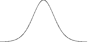
(b)
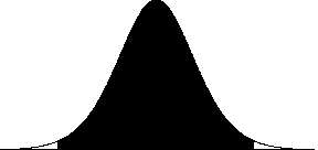
(c)
.025
(d)
2.201
(e)
greater
(f)
2.069
(g) 2.704
(h) 1.990
23-4: Exploring the t -Distribution ( cont. )
(a)
.1
(b)
between .025 and .01
(c)
between .025 and .01
(d)
between .025 and .01
(e)
between .005 and .001
(f)
less than .005
(g)
greater than .2
(h) between .010 and .002
23-5: Students' Sleeping Times ( cont. )
(a) - (c)
| Hypothetical sample | Sample size | Sample mean | Sample std. dev. | 95% confidence intervaL | (One-sided) p-value |
|---|---|---|---|---|---|
| 1 | 10 | 7.6 | 0.825 | 7.010, 8.190 | .080 |
| 2 | 10 | 7.6 | 1.597 | 6.457, 8.743 | .22 |
| 3 | 30 | 7.6 | 0.825 | 7.292, 7.908 | .0063 |
| 4 | 30 | 7.6 | 1.599 | 7.003, 8.197 | .091 |
(d)
Most accurate: 3;
Least accurate: 2;
Most evidence: 3;
Least evidence: 2
23-6: Students' Sleeping Times ( cont. )
(a) - (d) Answers vary.
(e)
The confidence interval would be narrower and the p-value smaller.
(f)
The confidence interval would be wider and the p-value larger.
(g)
The confidence interval would have the same width but be shifted down; the
p-value would be smaller.
(h) Answers vary.
(i)
No, since the fact that the students got up for an 8:00 am class would
affect the amount of sleep they got.

(a) - (c) These answers depend on class
results
(d)
Part of this answer depends on class
results. No, this proportion should not be close to 90% because
the
interval estimates the mean number of states visited in the
population and not individuals' values.
(e) cut in half
(f) decrease to one-third its original size
(g) not technically a simple random sample, but probably fairly representative
(h) The answer depends on class results.
24-2: Hypothetical ATM Withdrawals ( cont. )
(a)
| Sample size | Sample mean | Sample std. dev. | 95% confidence interval | |
|---|---|---|---|---|
| Machine 1 | 50 | 70.0 | 30.30 | (61.39, 78.61) |
| Machine 2 | 50 | 70.0 | 30.30 | (61.39, 78.61) |
| Machine 3 | 50 | 70.0 | 30.30 | (61.39, 78.61) |
(b) No, the distributions are very different.
(a)
| Couple # | Husband | Wife | Difference (husband - wife) |
|---|---|---|---|
| 1 | 25 | 22 | 3 |
| 2 | 25 | 32 | -7 |
| 3 | 51 | 50 | 1 |
| 4 | 25 | 25 | 0 |
| 5 | 38 | 33 | 5 |
| 6 | 30 | 27 | 3 |
| 7 | 60 | 45 | 15 |
| 8 | 54 | 47 | 7 |
| 9 | 31 | 30 | 1 |
| 10 | 54 | 44 | 10 |
| 11 | 23 | 23 | 0 |
| 12 | 34 | 39 | -5 |
| 13 | 25 | 24 | 1 |
| 14 | 23 | 22 | 1 |
| 15 | 19 | 16 | 3 |
| 16 | 71 | 73 | -2 |
| 17 | 26 | 27 | -1 |
| 18 | 31 | 36 | -5 |
| 19 | 26 | 24 | 2 |
| 20 | 62 | 60 | 2 |
| 21 | 29 | 26 | 3 |
| 22 | 31 | 23 | 8 |
| 23 | 29 | 28 | 1 |
| 24 | 35 | 36 | -1 |
(b)

(c)
 = 1.875;
s = 4.812
(d)  :
:  = 0
= 0
 :
:  > 0
> 0
t = 1.91
p-value = .034
(e)
(.191, 3.559)
(f) (Asks for interpretation)
24-4: Planetary Measurements ( cont. )
(a)
(71.22, 2132.78)
(b)
No, the interval is senseless since the data do not constitute a sample
from a population.

(a) no
(b) Yes, route 1 seems to be quicker.
(c)
| Sample Size | Sample mean | Sample standard deviation | |
|---|---|---|---|
| Alex 1 | 10 | 28 | 6 |
| Alex 2 | 10 | 32 | 6 |
(d)
| Sample Size | Sample mean | Sample standard deviation | Two-sided p-value | |
|---|---|---|---|---|
| Alex 1 | 10 | 28 | 6 | .15 |
| Alex 2 | 10 | 32 | 6 |
(e)
no;
no;
the observed difference in times is not unlikely to have occured by
chance.
(f)
Barb's centers are farther apart.
(g)
Carl's times are less spread out.
(h)
Donna has larger samples of times.
(i)
| Sample Size | Sample mean | Sample standard deviation | Two-sided p-value | |
|---|---|---|---|---|
| Barb 1 | 10 | 25 | 6 | .0017 |
| Barb 2 | 10 | 35 | 6 | |
| Carl 1 | 10 | 28 | 3 | .0080 |
| Carl 2 | 10 | 32 | 3 | |
| Donna 1 | 40 | 28 | 6 | .0038 |
| Donna 2 | 40 | 32 | 6 |
(j)
Barb's sample means are farther apart;
Carl's sample times are less variable (smaller standard deviation);
Donna has larger samples of times.
25-2: Students' Haircut Prices
(a) - (e) These answers depend on class results.
25-3: Trading for Run Production
(a) raw data (at least sample sizes and standard deviation)
(b)
| Minimum | Lower quartile | Median | Upper quartile | Maximum | |
|---|---|---|---|---|---|
| Without McGriff | 0 | 2 | 3 | 5 | 13 |
| With McGriff | 0 | 3 | 5 | 8 | 18 |
(c)
| Sample size | Sample mean | Sample standard deviation | |
|---|---|---|---|
| Without McGriff | 94 | 3.989 | 3.074 |
| With McGriff | 68 | 5.779 | 3.816 |
(d)
t = -3.19;
p-value = .0018
(e)
no
(f) no; this is an observational study